Introduction Take notes for the advanced algorithm and write down the knowledge points in each chapter

Advanced Algorithm

Course preview

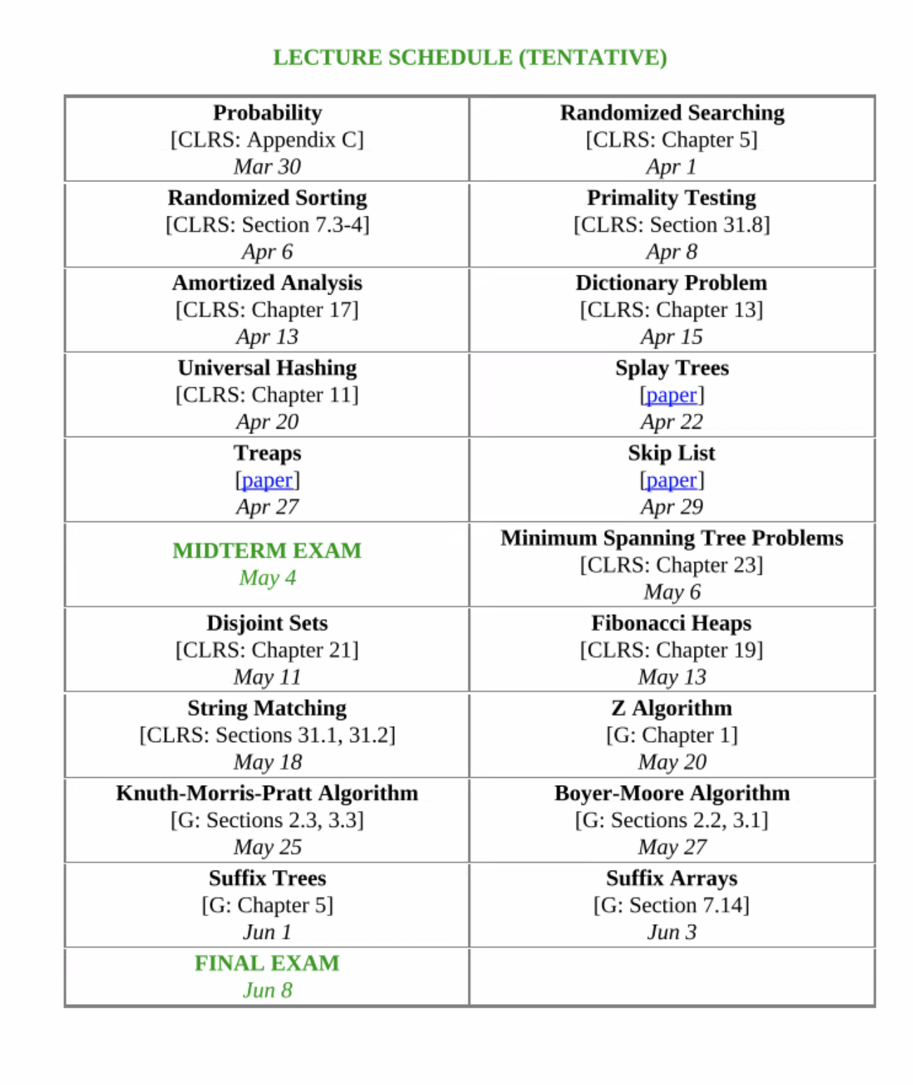
Lecture schedule

Summary

Four old problems

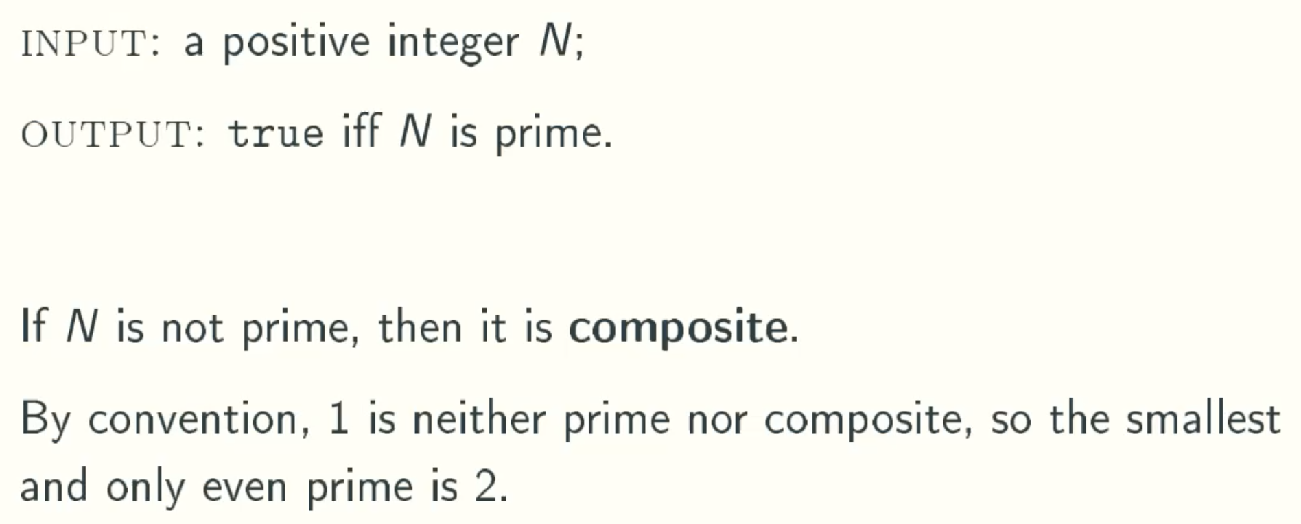
• primarily testing: determine if a given integer is prime
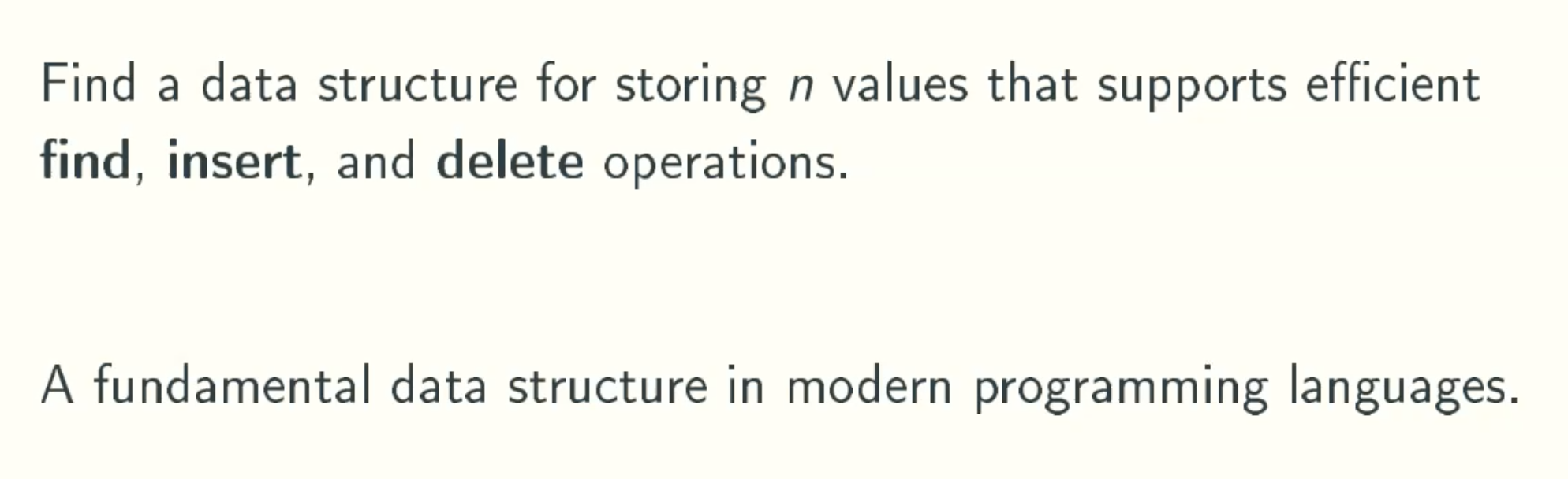
• dictionary problem: design an efficient data structure that support find, insert, and delete operations
• minimum spanning trees
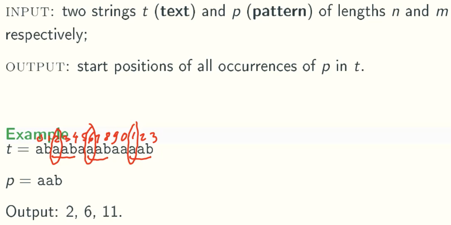
• string matching: find all occurrences of a pattern string p in a text string t

Two new tools

• randomized algorithms: have access to a random source
• amortized analysis: worst-case analysis of a sequence of operations

Primarily Testing

Problem defination

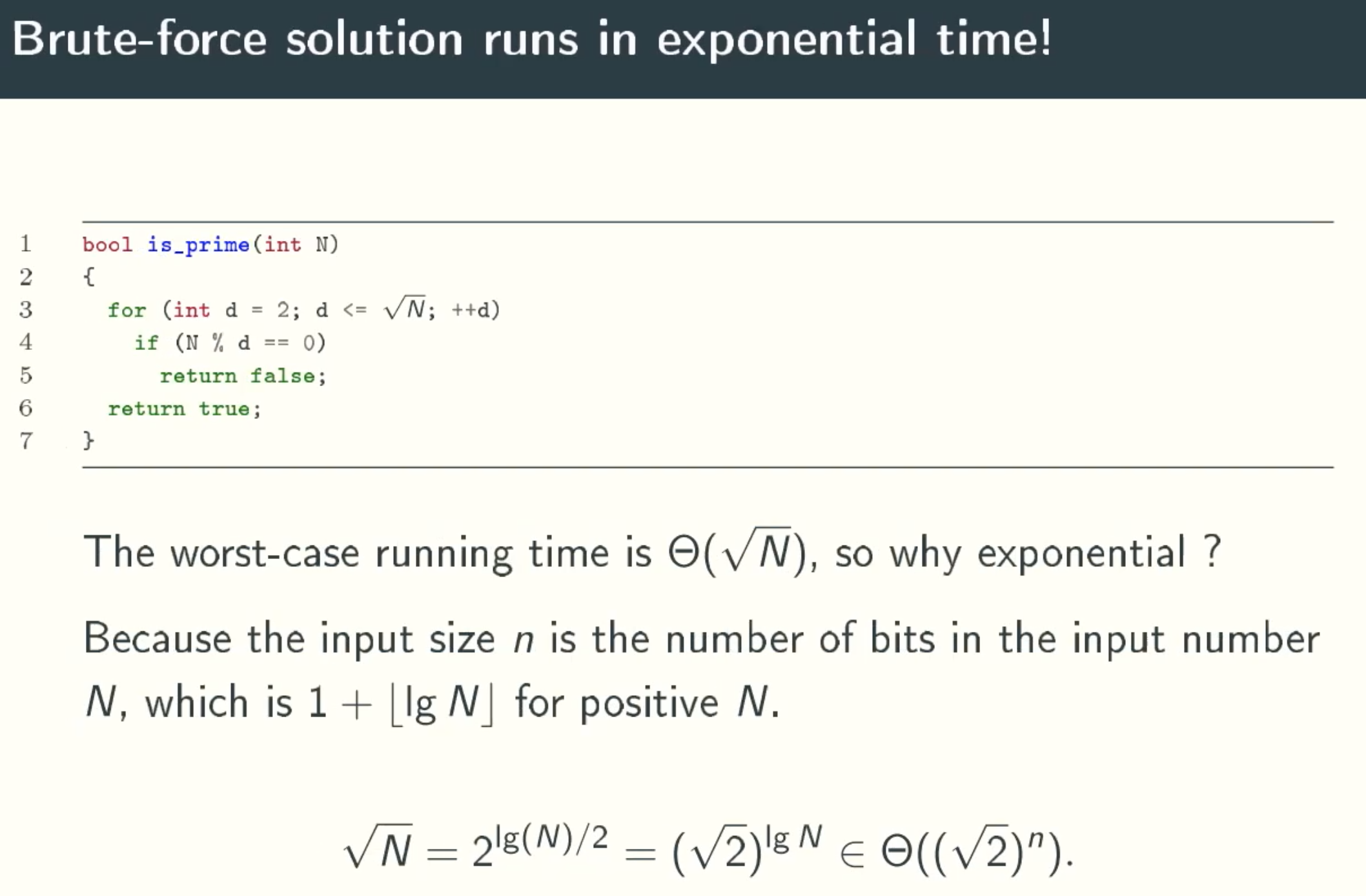
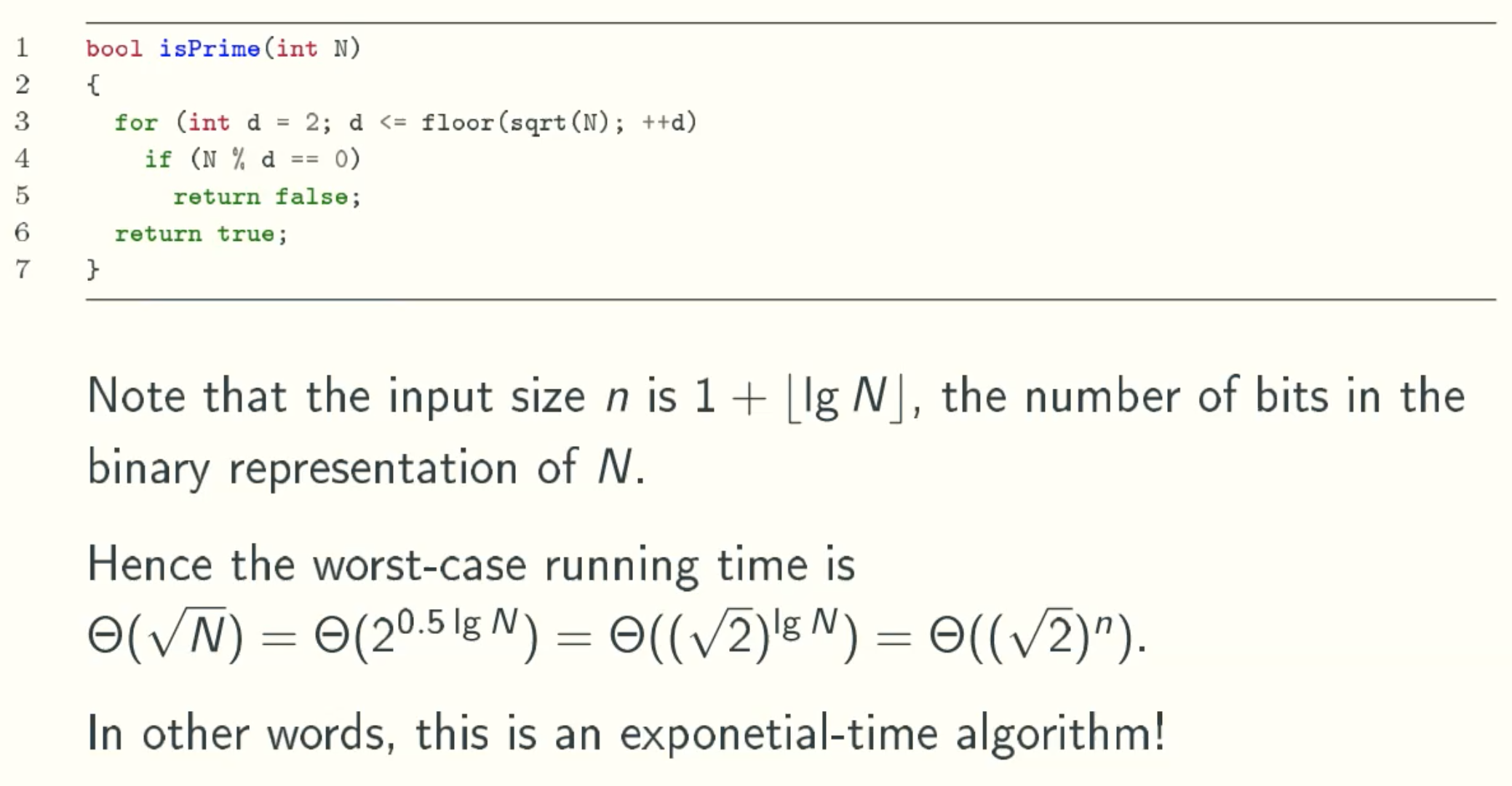
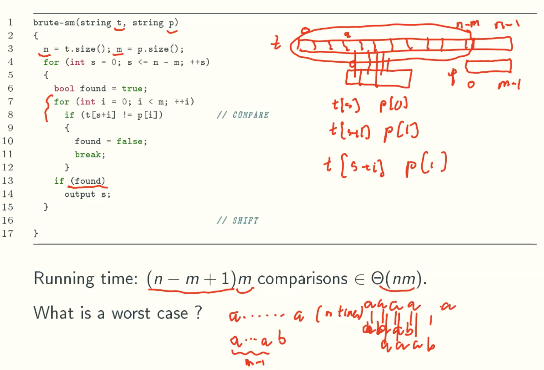
brute-force solution

Q & A:

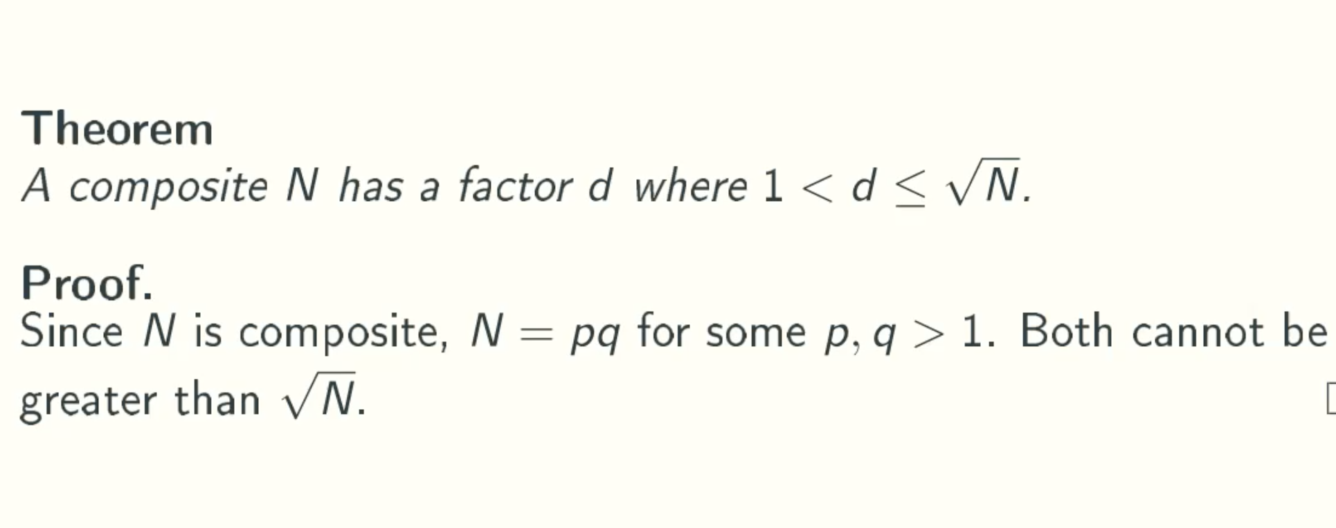
1. why the loop is from 2 to √n
   A prime number is a number that is not divisible by any number other than itself and 1. Therefore, we start from 2. And this loop is to check whether there is a pair p * q = n = √n * √n, therefore, the smaller one in p and q musct smaller or equal than √n. So the iteration from 2 to √n will cover all possibilities.

2. why √N = 2^(lg(N)/2)
   √N = 2^(lg(√N)) = 2^{(lg (N1/2))} = 2^(1/2*lg(N))

3. why (√2)^lgN = √2ⁿ
   n is the binary bit of this N

N	lgN + 1	n
1	lg1 + 1	1
2	lg2 + 1	2
3	lg3 + 1	2
4	lg4 + 1	3
5	lg5 + 1	3

And let’s think of lgN + 1 as lgN, we dismiss plus 1 here where N is big enough.

4. why this algorithm is exponential?
   the running time is θ((√2)ⁿ), n is the bit of value N, and we look n here is input size. Therefore, the running time is exponential.

Dictionary Problem

Problem defination

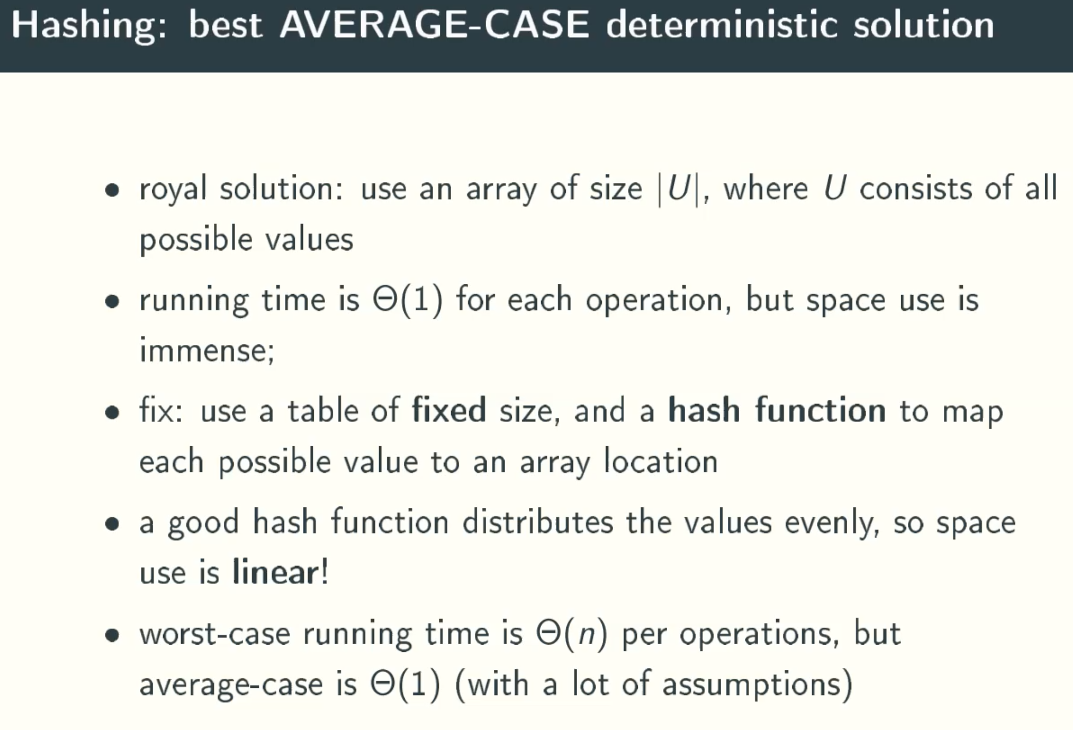
O(1) Time & O(n) Space solution

BST solution

note
BST: binary serach tree, quite slow in reality.
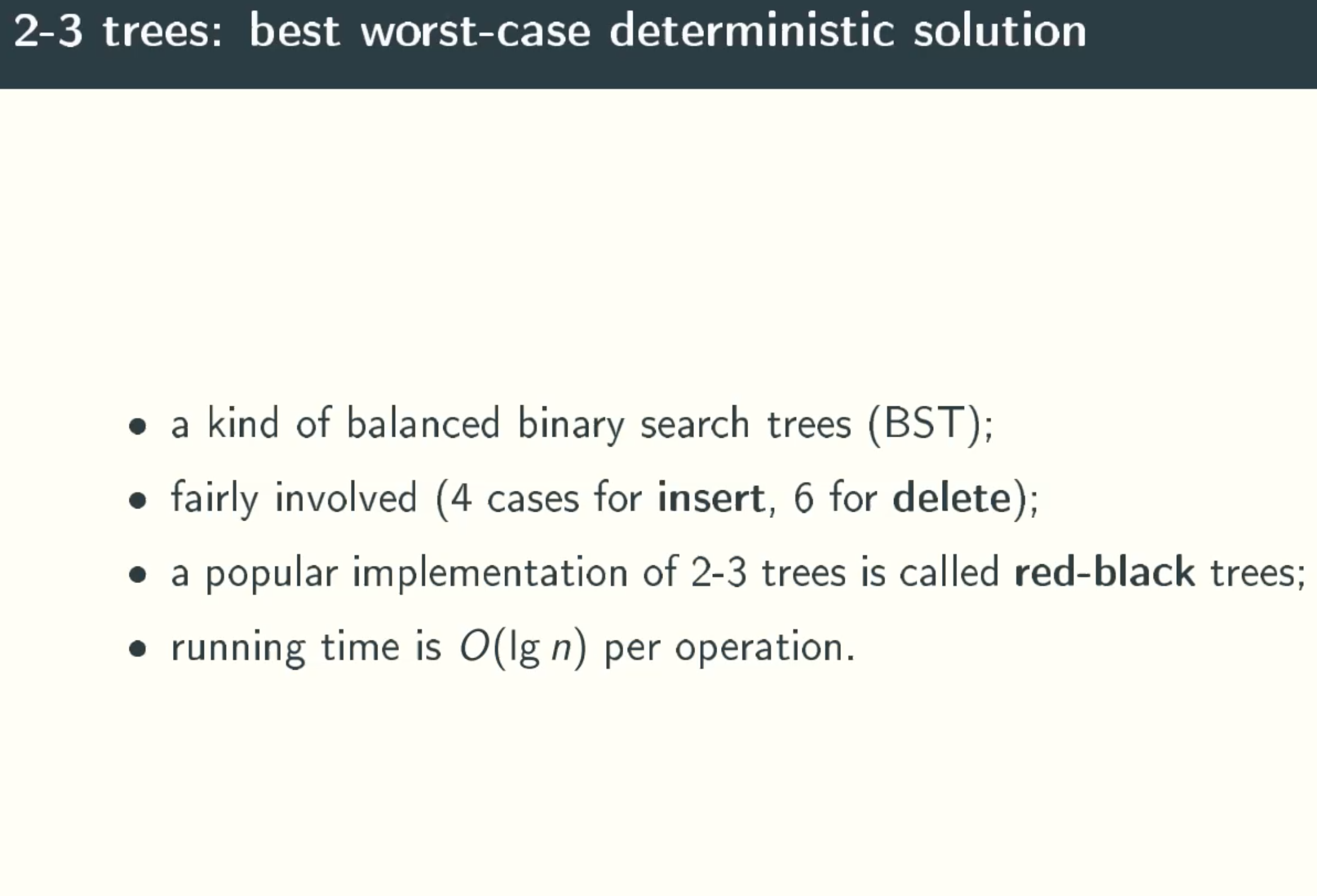
2-3 Tree: a tree whose nodes can have two or three children nodes. Hard to implement.

New solution

• splay tree: amortized BST
  When a node x is accessed, a splay operation is performed on x to move it to the root. To perform a splay operation we carry out a sequence of splay steps, each of which moves x closer to the root. By performing a splay operation on the node of interest after every access, the recently accessed nodes are kept near the root and the tree remains roughly balanced, so that we achieve the desired amortized time bounds.
• treaps: randomized BST
  Treap = Tree + Heap. Treap itself is a binary search tree, its left subtree and the right subtree are also a Treap, and the common binary search tree is different, Treap records an additional data, is the priority. Treap not only forms a binary search tree with key codes, but also satisfies the property of heap. Treap’s approach to maintaining heap properties uses rotations, which require only two rotations and are less programming complicated than Splay’s.
• skip lists: randomized linked lists
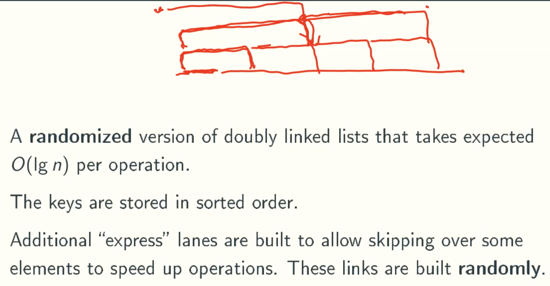
  normal linked list: insert & delete O(1), checkO(n)
  Skiplist uses the idea of space for time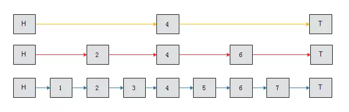
  
  use binary search improve search efficiency.
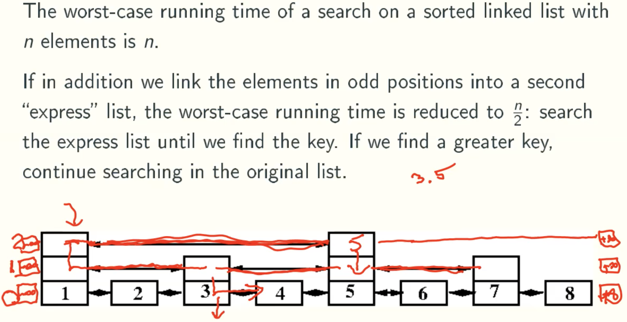
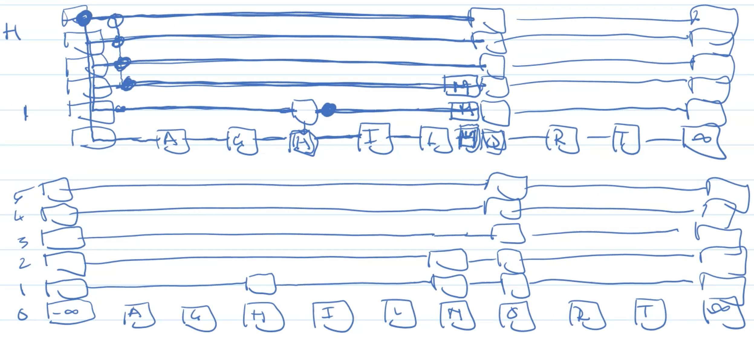
  the blew one is original linked list, the middle one is original list divided into four parts, the top one is original list divided into two parts. And if we want to search 7.
  the original search range is (H, T)

1. in the top list, 7 > 4, search range becomes (4, T)
2. in the middle list, 7 > 6, search range becomes (6, 7)
3. in the below list, 7 == 7, search success!

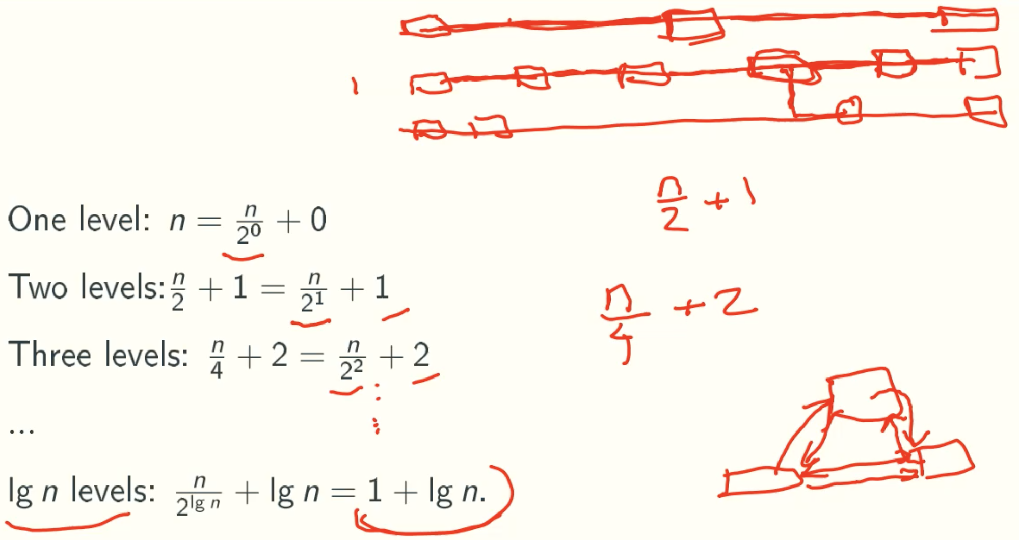
In general, Skiplist stores additional intermediate information for binary lookups

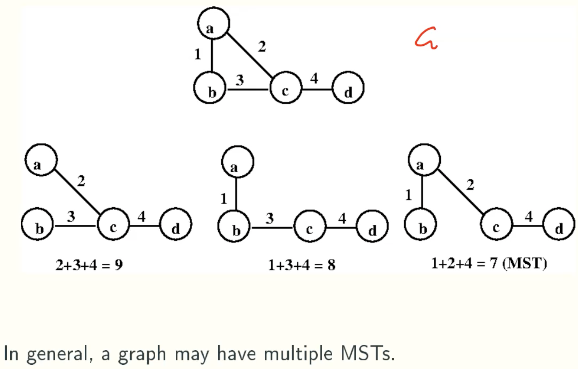
Minimum Spanning Trees

Problem defination

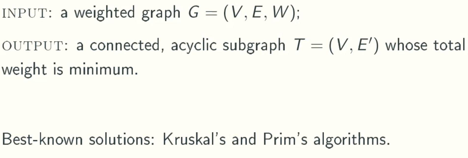
connect all nodes, no cycle, minimum weight

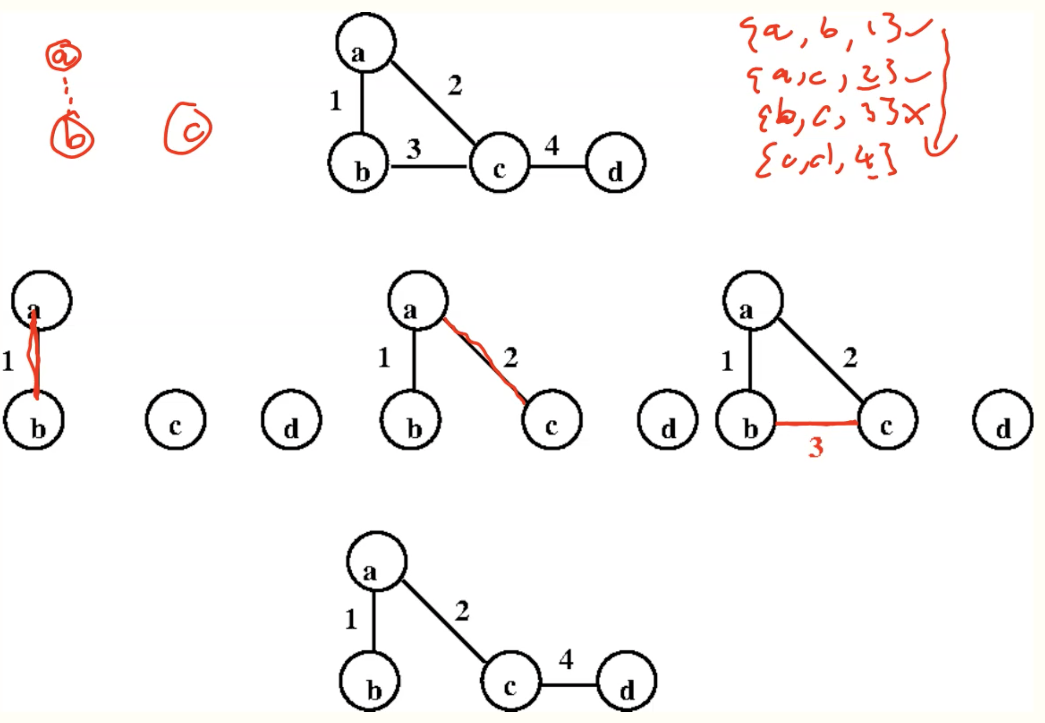
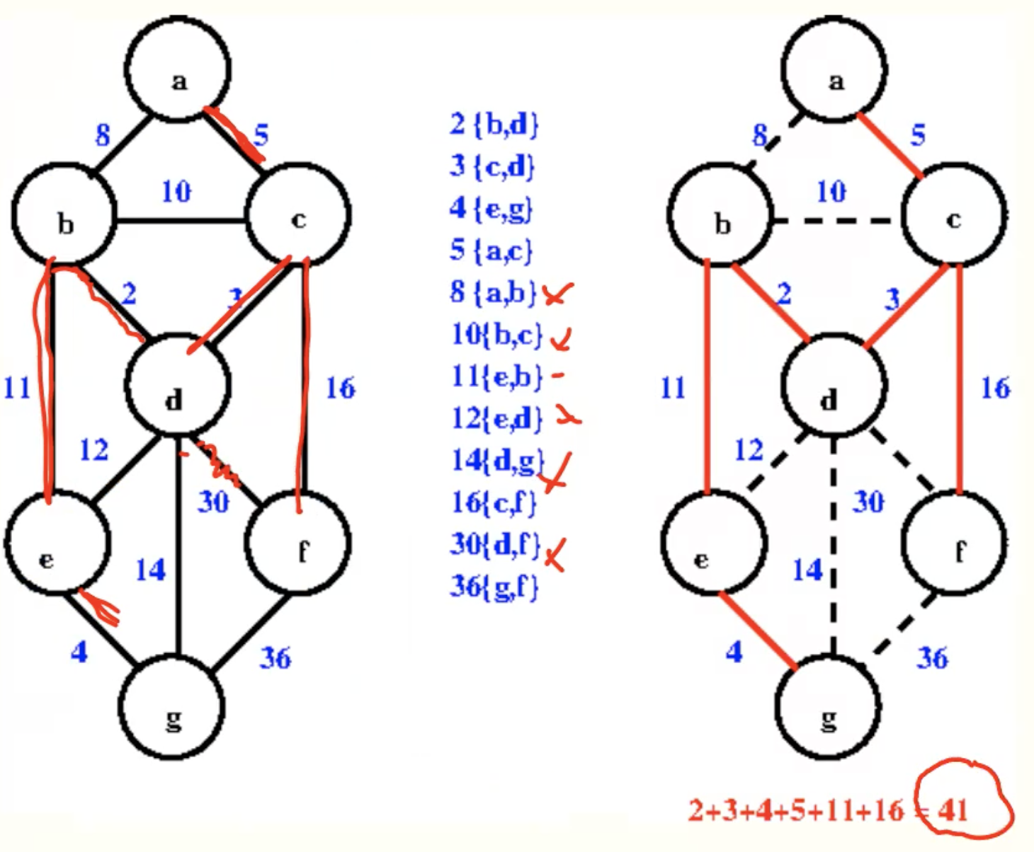
Kruskal algorithm

Algorithm introduction

sort weight ascendingly, iterate every edge, if the nodes on the edge is in different group, use this edge and let one node join the other.

Prim algorithm

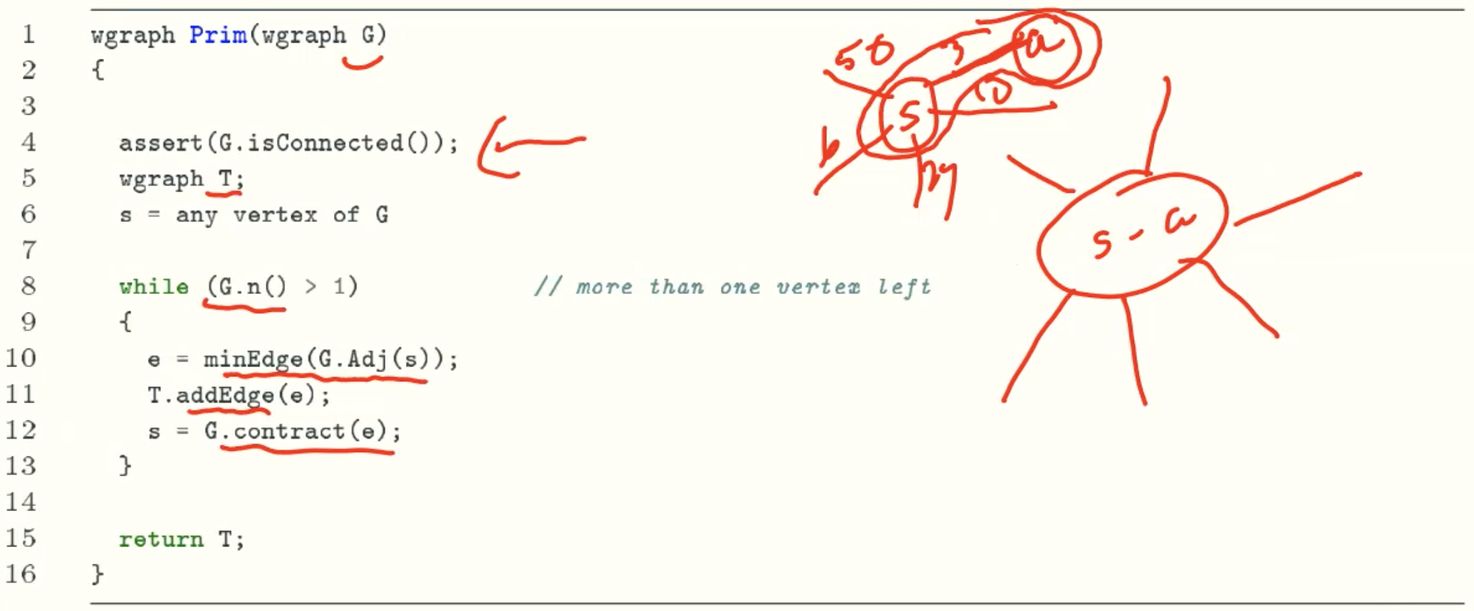
Algorithm introduction

1. Add one node to the set V

2. while(not all nodes in set V) {

   • find the least weighted edge from the nodes in the set V to the nodes outside the set
   • then add this edge and this outer node to the set V
     }

Disjoint set

alias: Union-find

Fibonacci heap

A Fibonacci heap is a collection of trees satisfying the minimum-heap property, that is, the key of a child is always greater than or equal to the key of the parent. This implies that the minimum key is always at the root of one of the trees.

String Matching

Problem defination

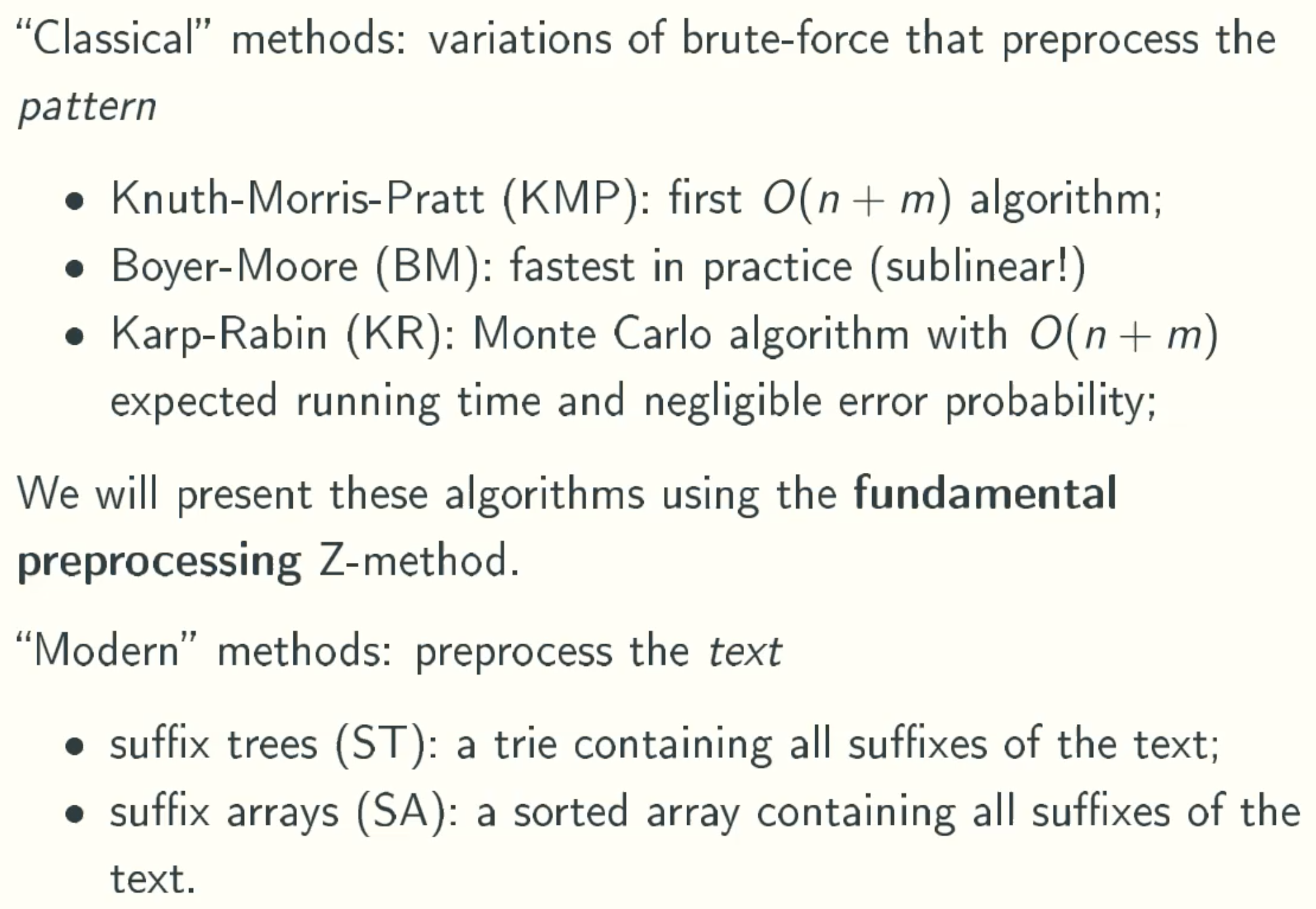
Classic solutions

• variations of brute-force algorithm, θ(mn);
• KMP(Knuth-Morris-Pratt) algorith, first θ(m + n);
• Boyer-Moore is the fastest in practice;
• Karp-Rabin runs in expected θ(n+m);
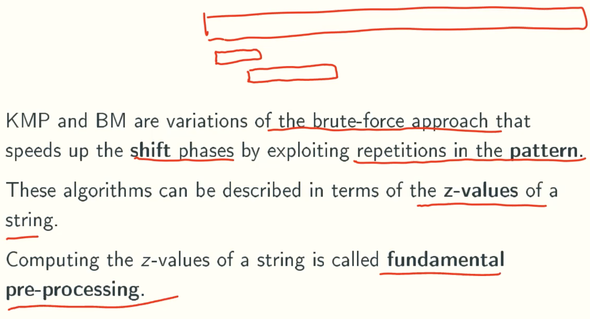
• Z algorithm a new preprocessing technique that underlies both KMP and BM;
• These modifications preprocess the pattern;

Generating Random Sequences Of Integers

Desirable properites of rand(n)

• not truly random, but only appears random according to various statistical tests(such as equal number of 0, …, n - 1 in a long generated sequence)
• efficiently computable and determinstic(reproducible)

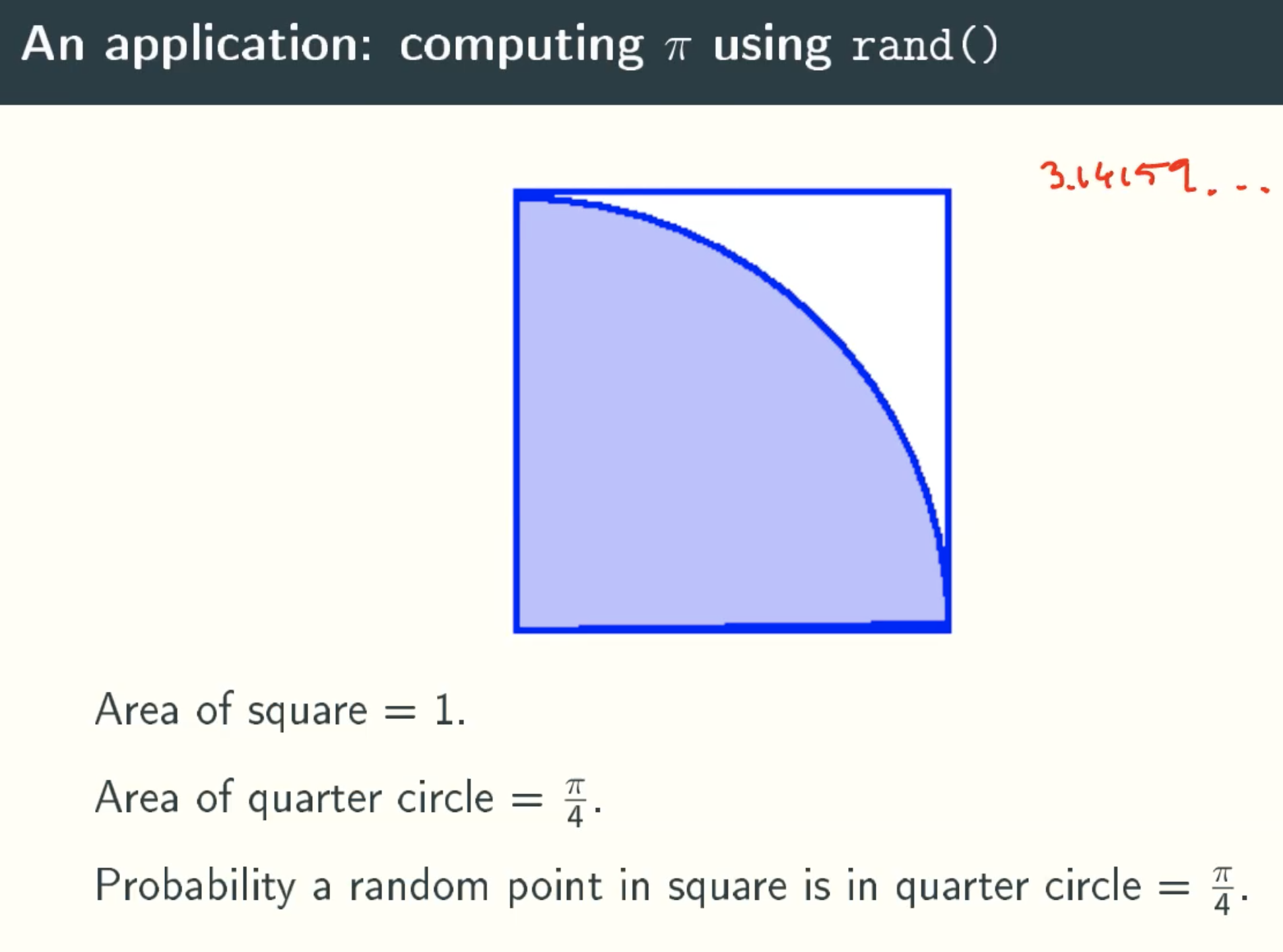
Computing ∏ using rand()

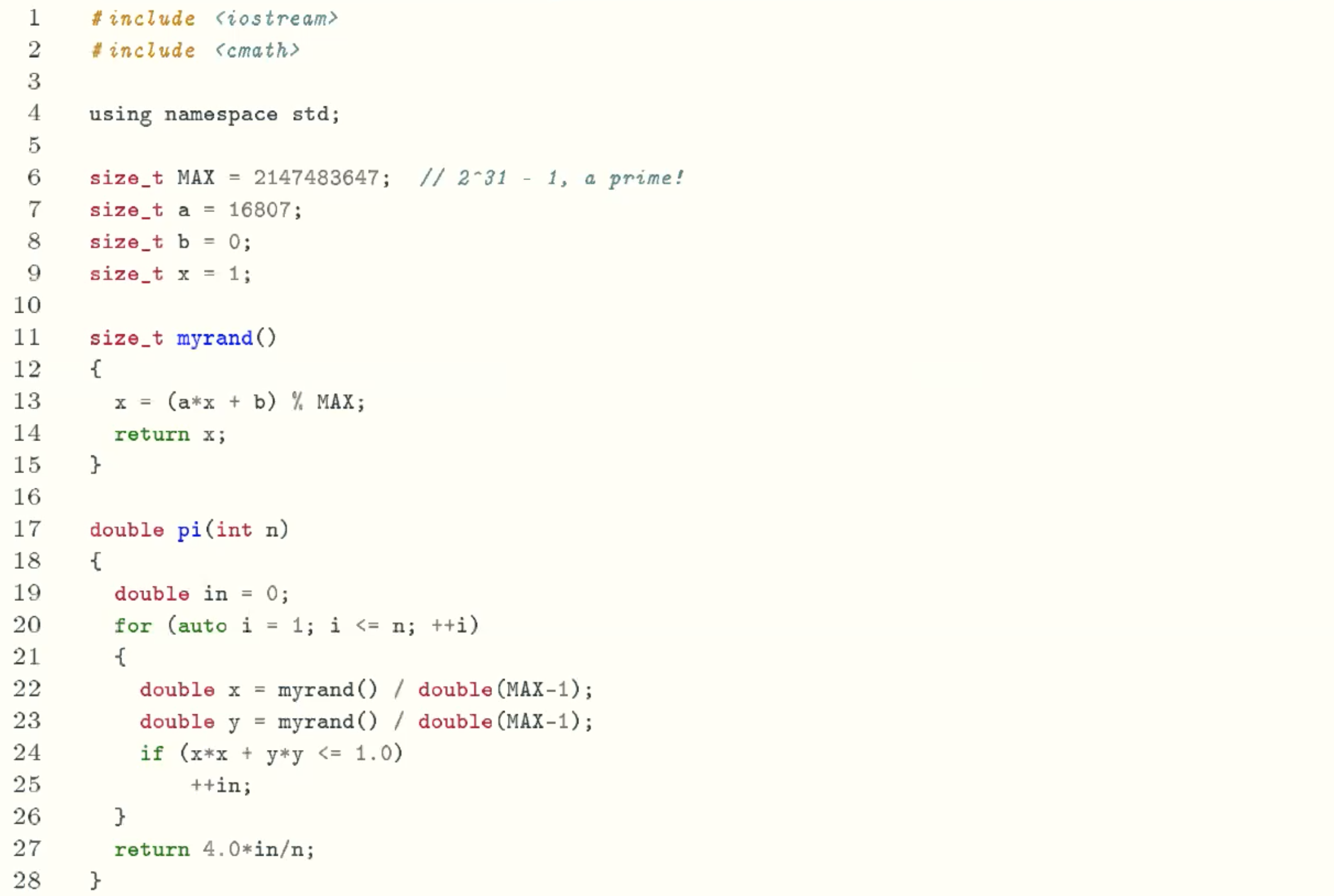
Implementation

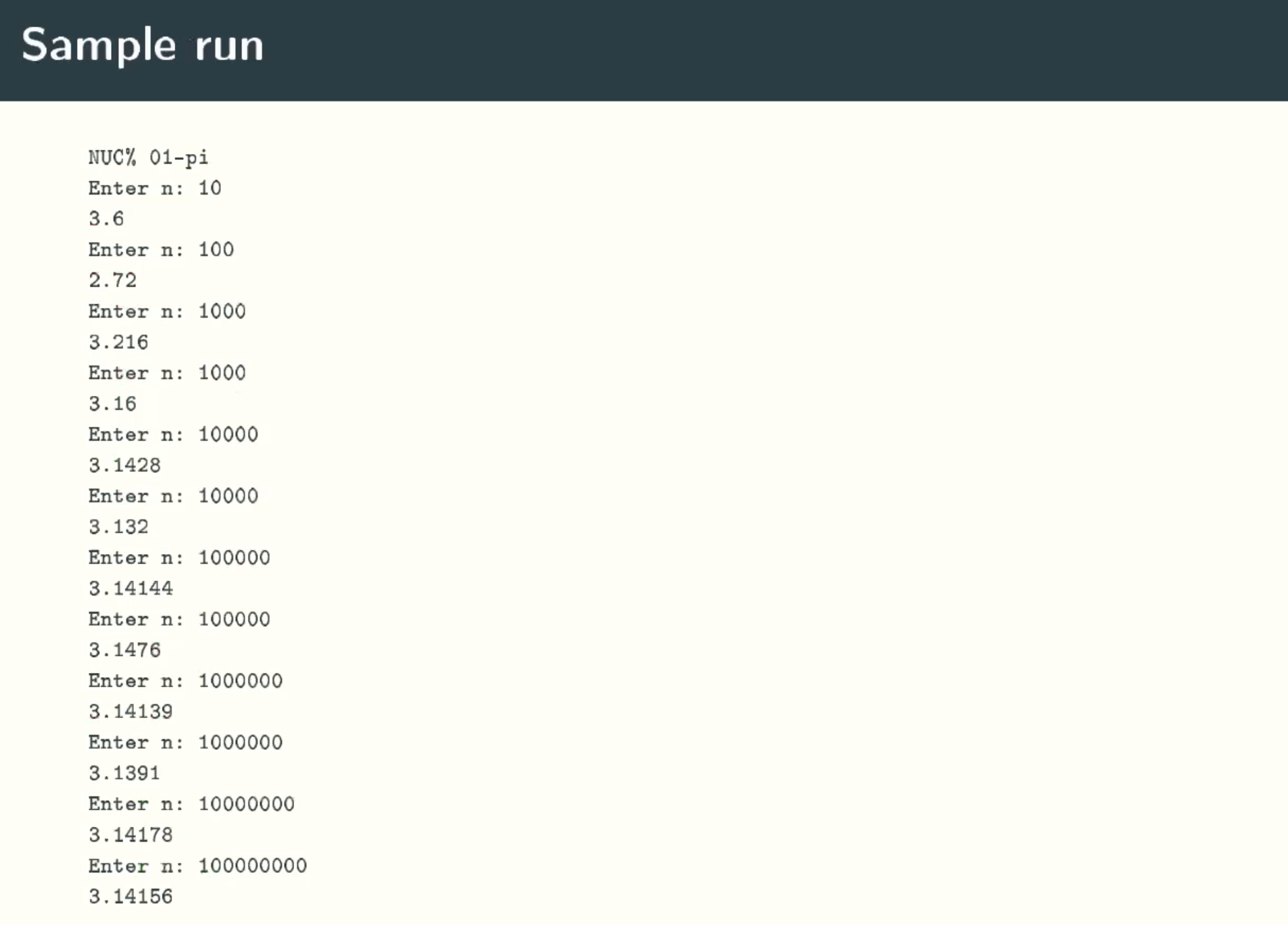
Sample run

Randomized Algorithm

Review of probability theory

Random Variables

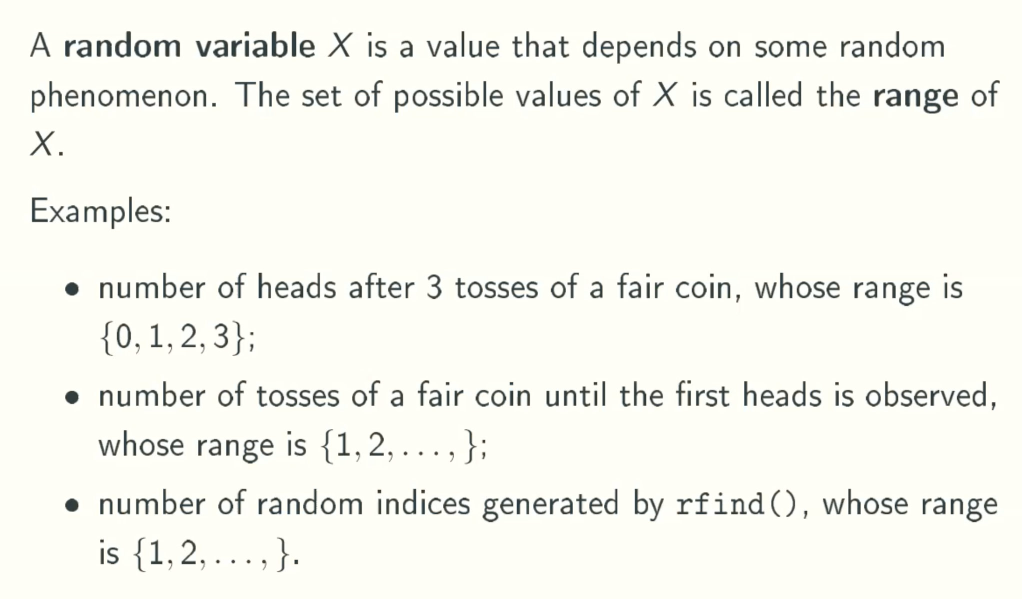
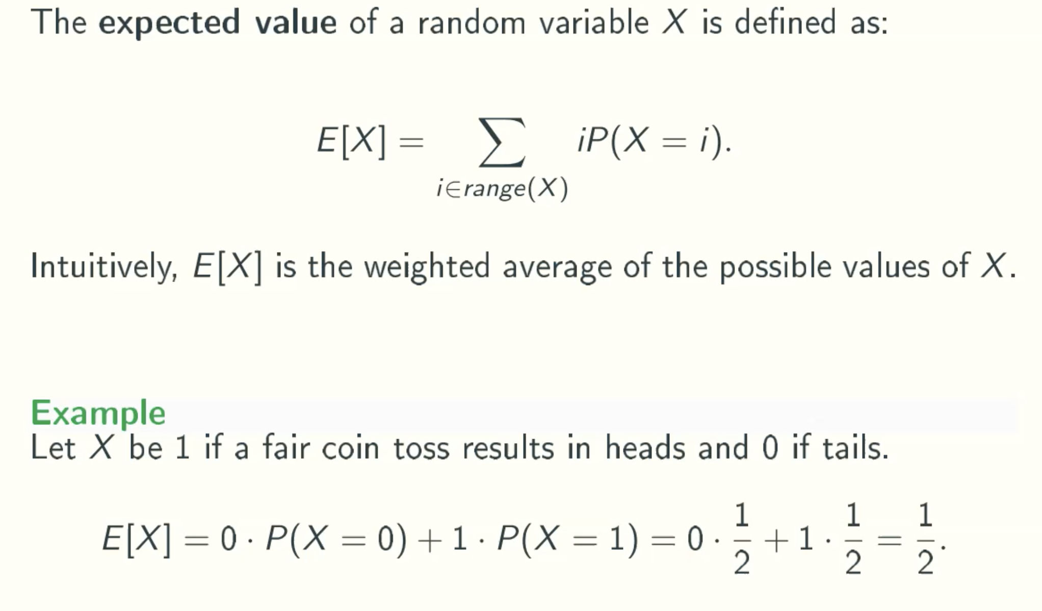
Expected Value

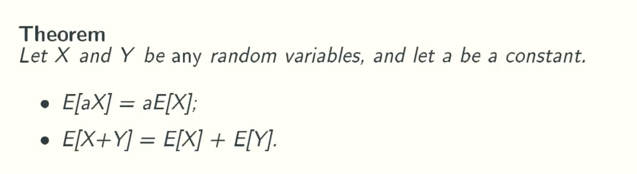
Linearity Of Expected Values

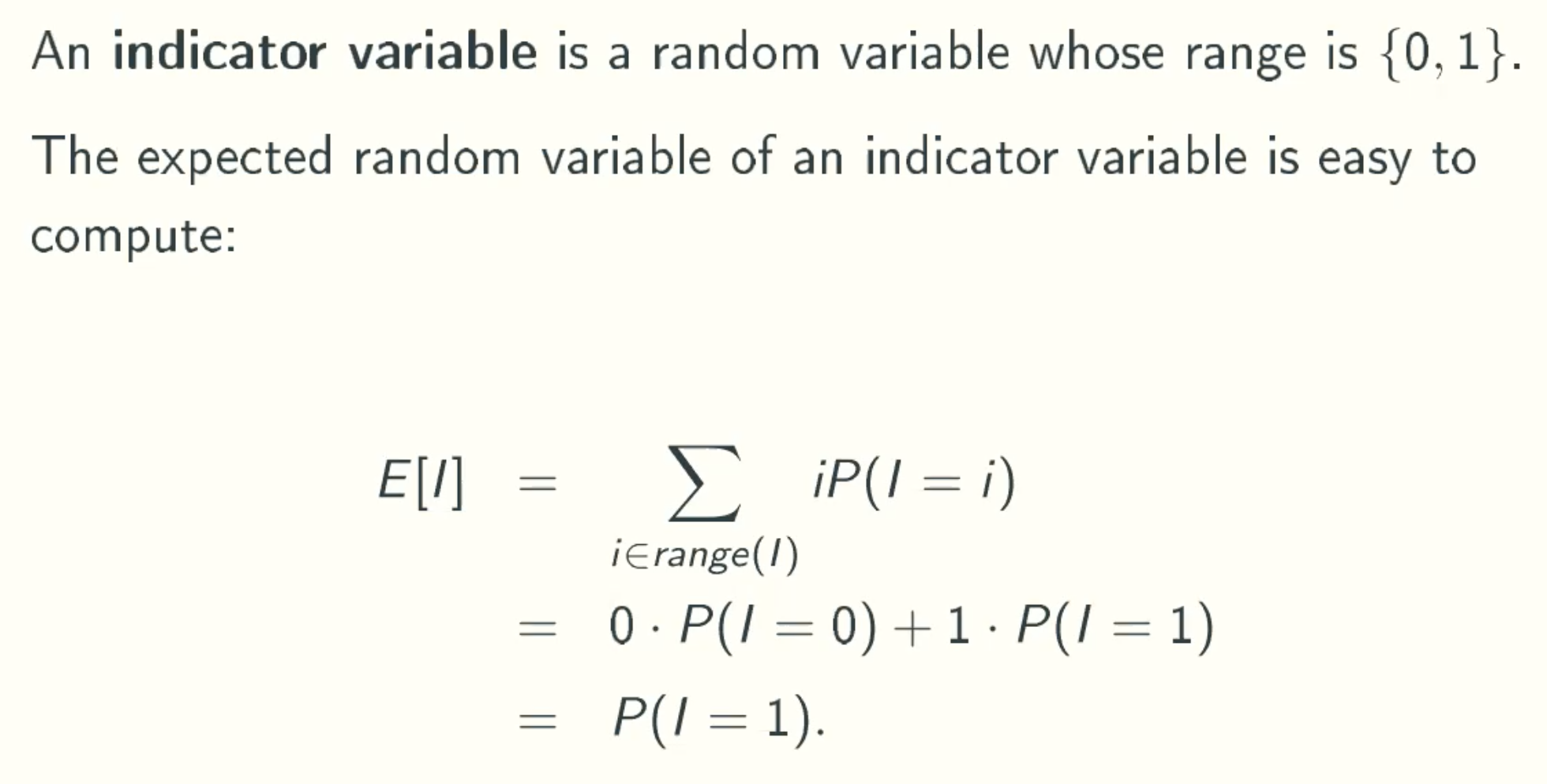
Indicator Random Variables

Example 1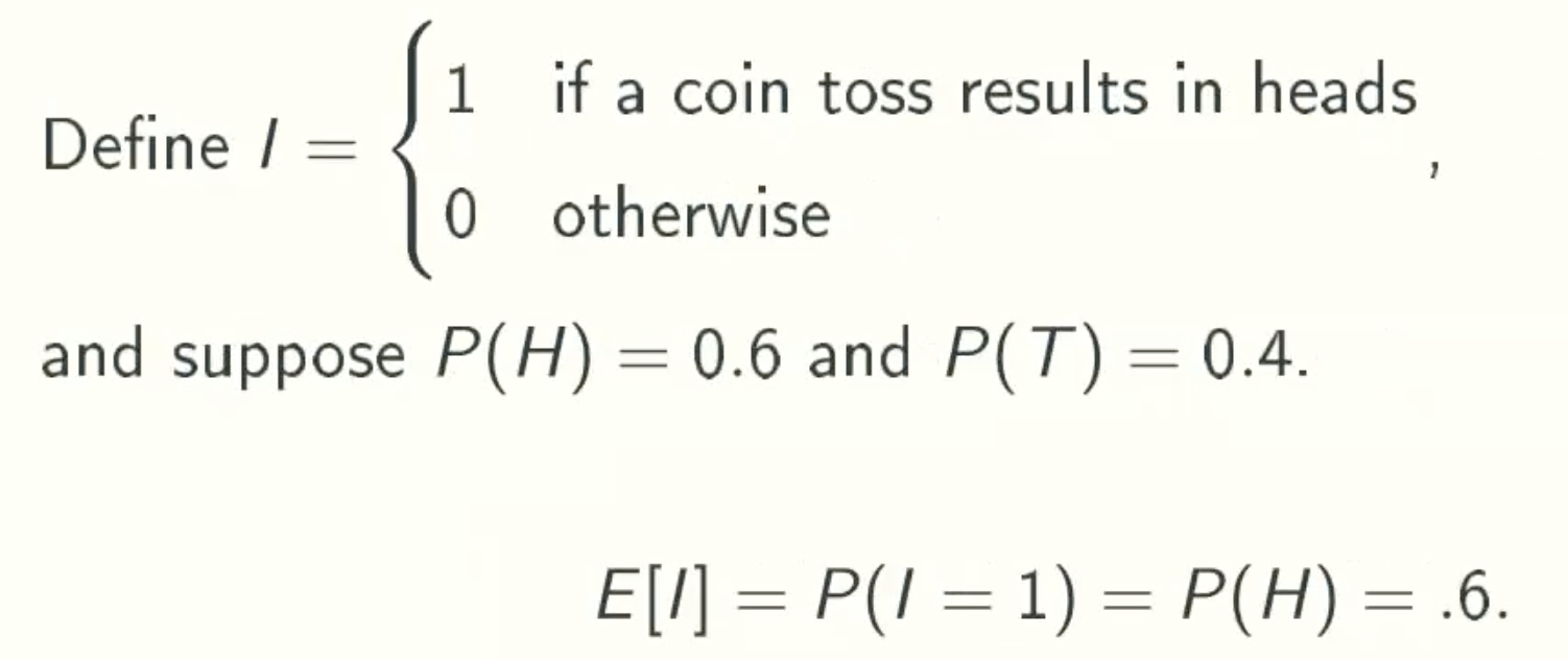

Example 2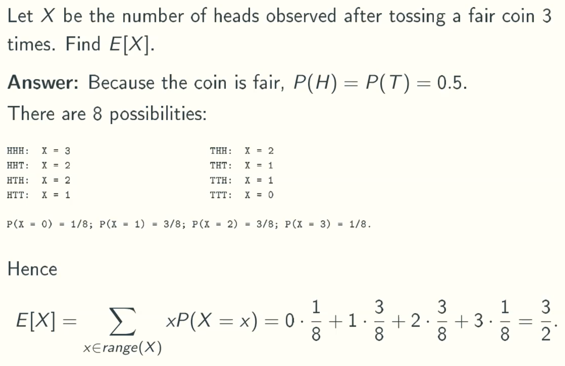

Simpler Solution using linearlity of expected values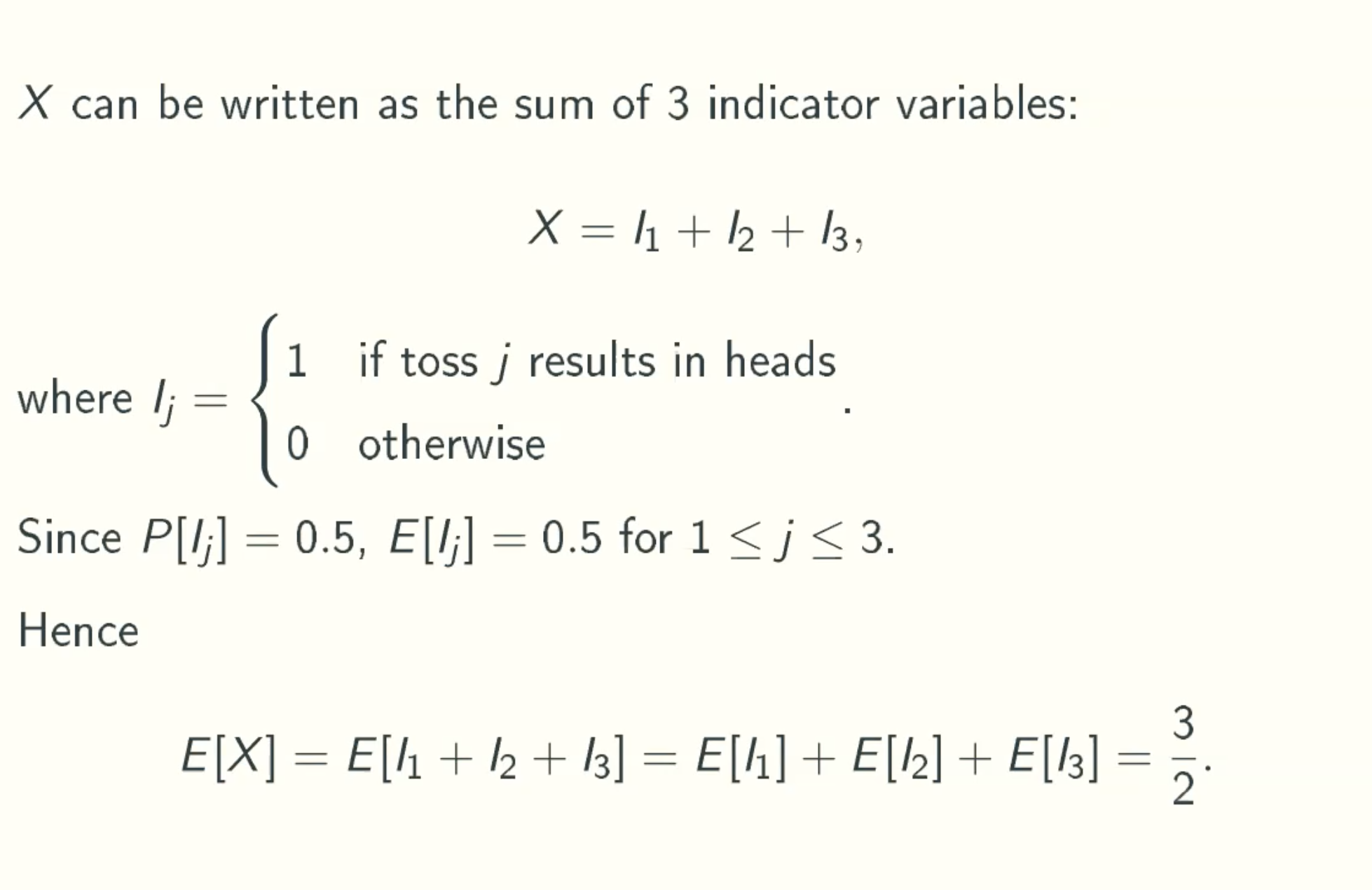

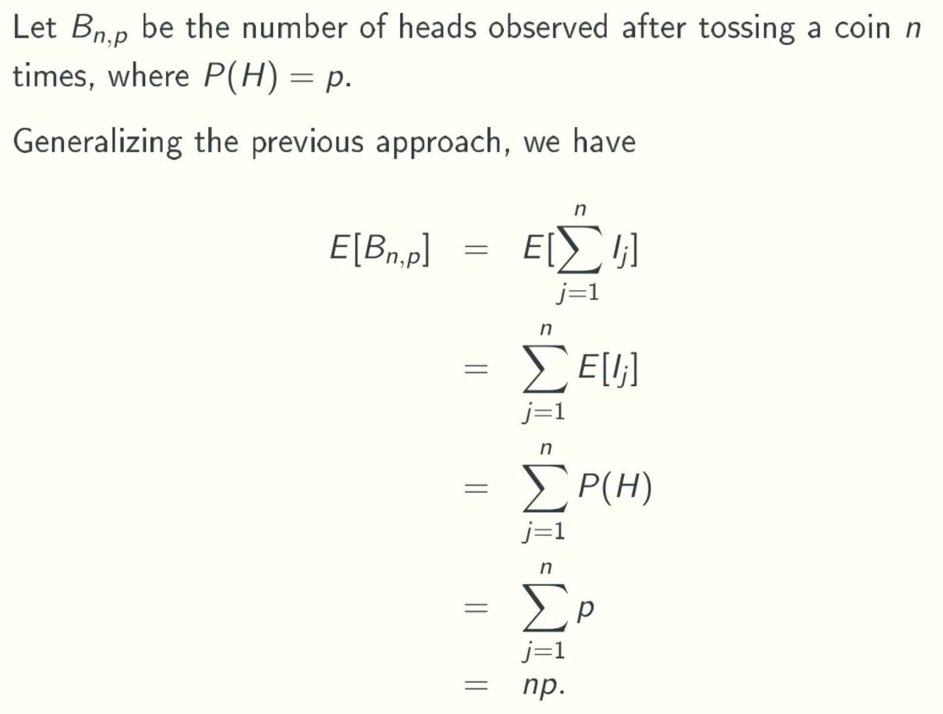
Binomial Random Variable B_n,p

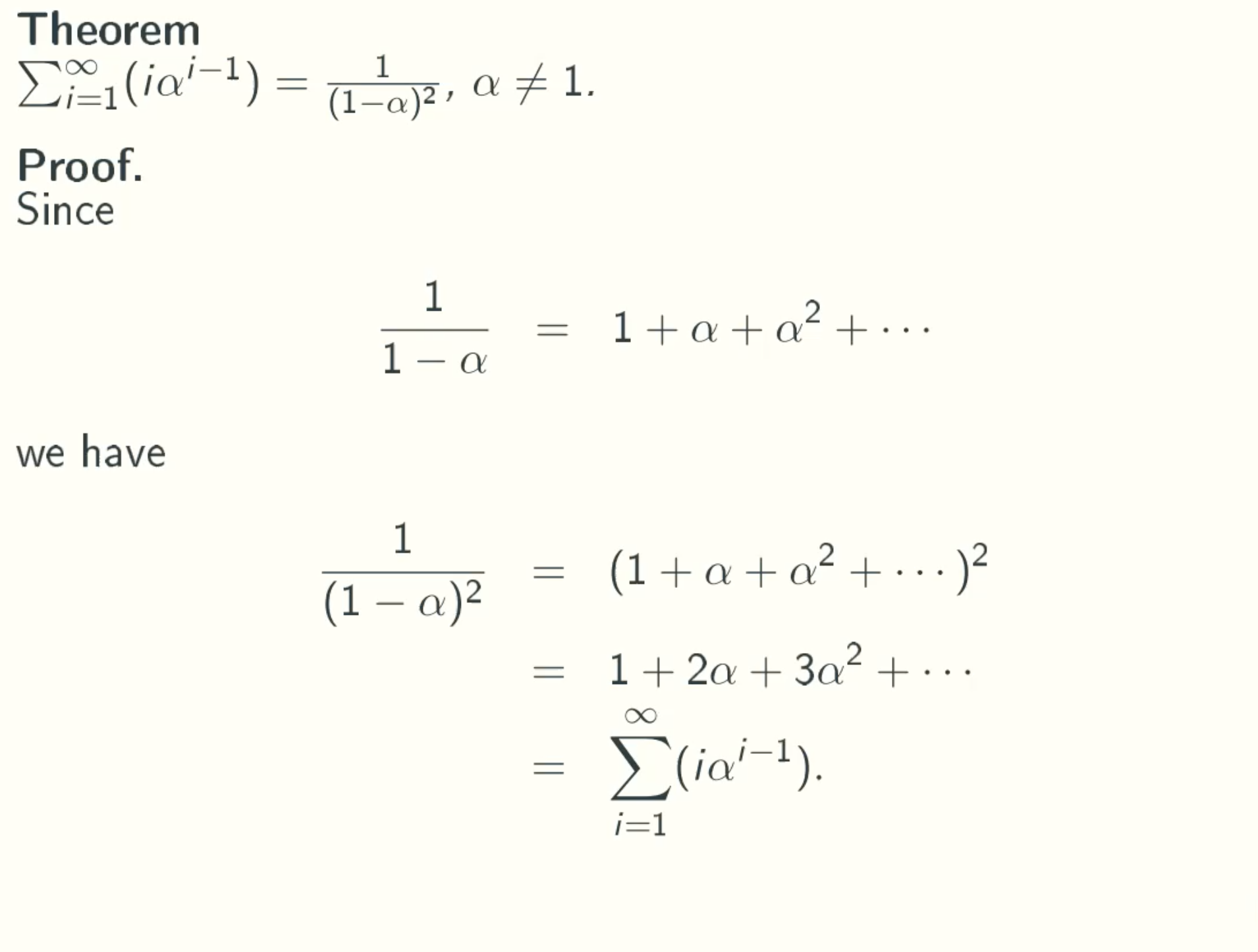
An Infinite Sum

note:
since 1/(1-a) = 1 + a + a² + a³ + …
(1/(1/a))² = (1 + a + a² + a³ + …)²
= 1 + a + a² + a³ + …

• 0 + a + a² + a³ + …
• 0 + 0 + a² + a³ + …
• 0 + 0 + 0 + a³ + …
• …
  = 1 + 2a + 3a² + 4a³ + …
  = ∑(i=1-∞)ia^i-1

​

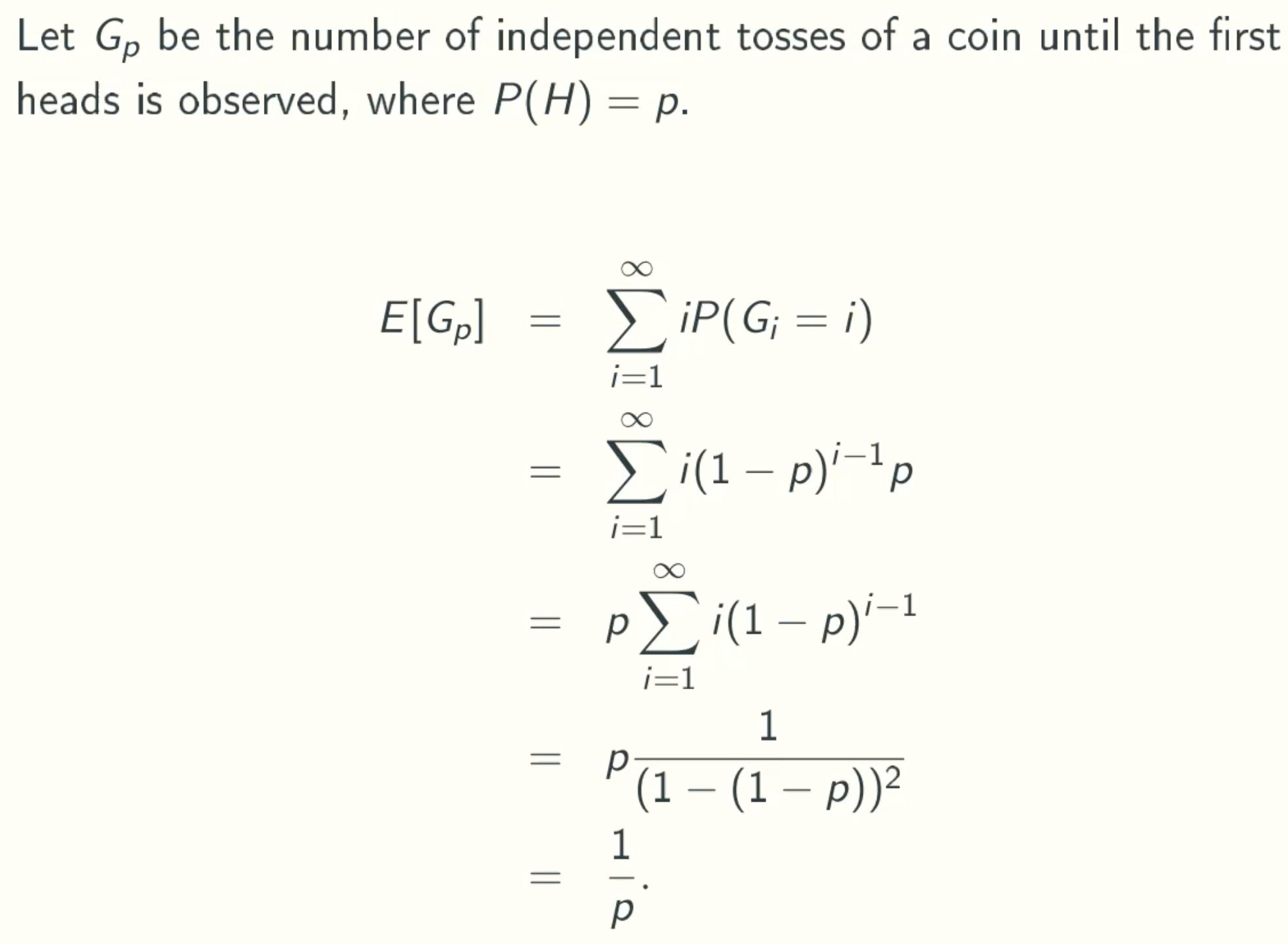
Geometric random variables G_p

Q&A
why p∑i(1-p)^i-1 = p / (1 - (1 - p))²
because theorem ∑ia^i-1 = 1 / (1-a)² a ≠ 1

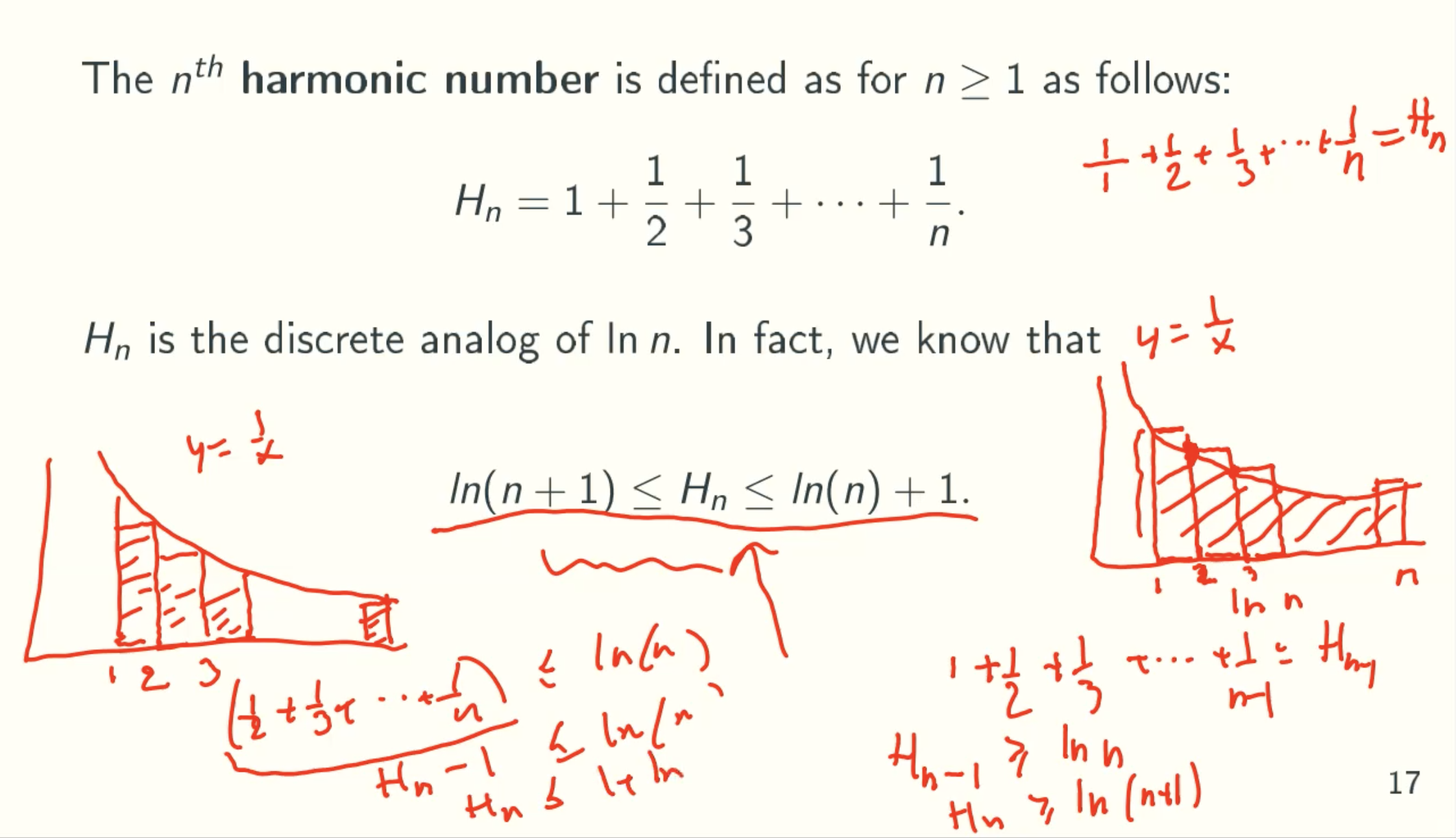
Harmonic Numbers

Q&A:

1. Why H_n ≥ ln(n+1)
   use the upper bound to calculate rectangle area
   area = 1 + 1/2 + 1/3 + … + 1/(n-1) = H_n-1
   And ln(n) is under area of this curve, since (ln(n))’ = 1/n
   therefore, H_n-1 ≥ ln(n), then replace n with n+1, we get H_n ≥ ln(n+1)
2. Why H_n ≤ ln(n) + 1
   use the lower bound to calculate rectangle area
   area = 1/2 + 1/3 + … + 1/n = H_n - 1
   And ln(n) is under area of this curve, since (ln(n))’ = 1/n
   therefore, H_n - 1 ≤ ln(n), H_n ≤ ln(n) + 1

Randomized Searching

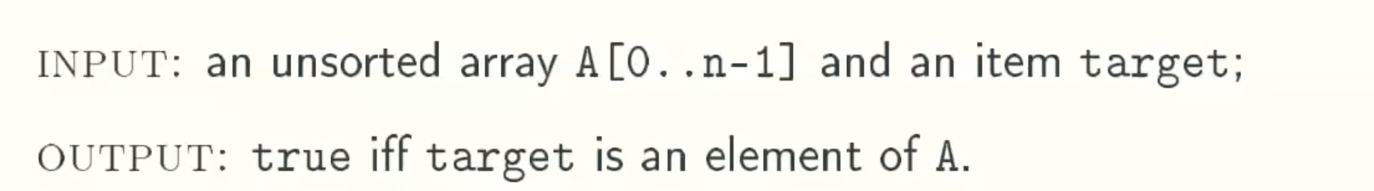
Problem defination

Deterministic Solution

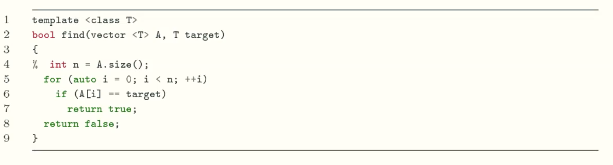
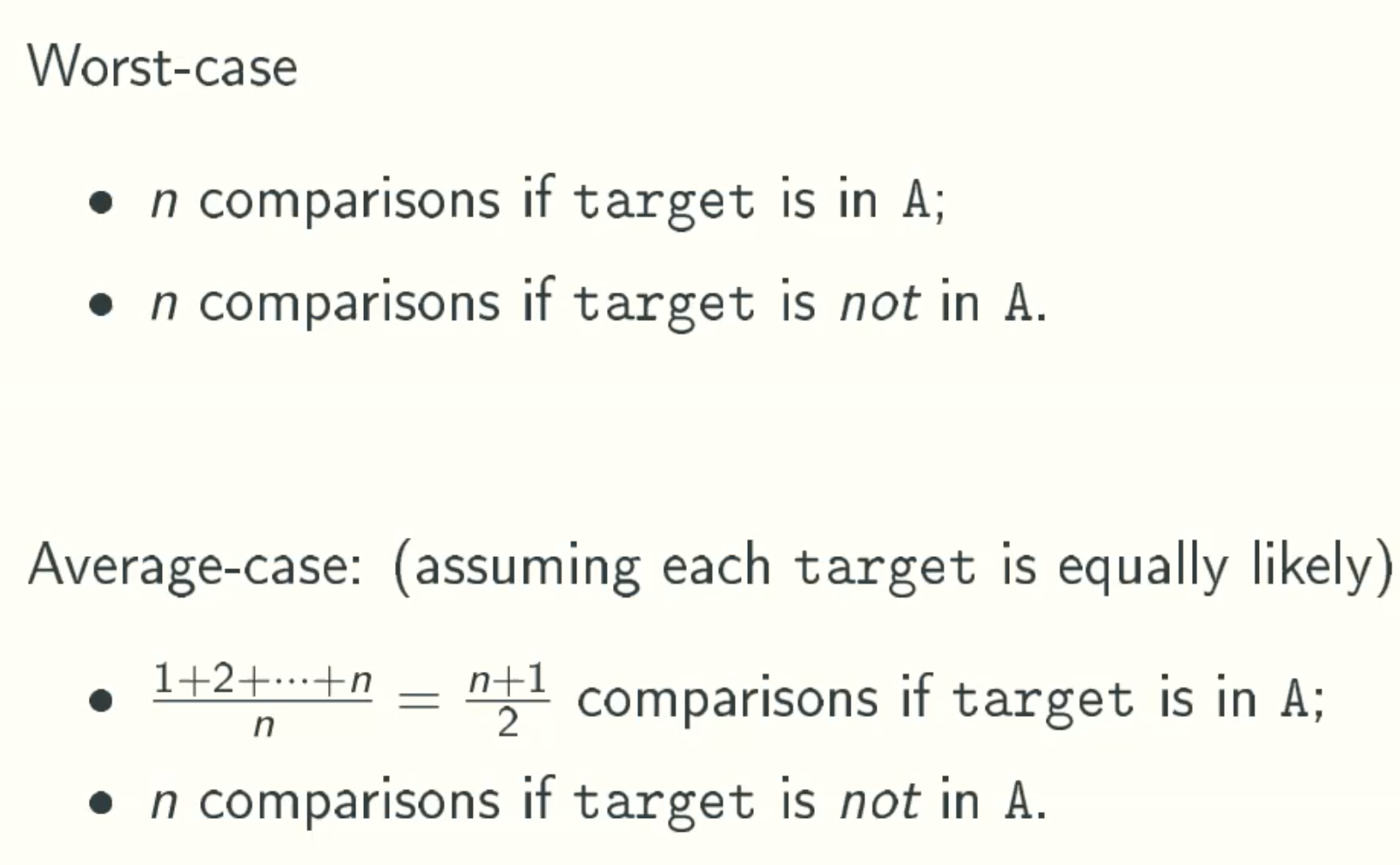
Solution Analysis

Randomized Solution

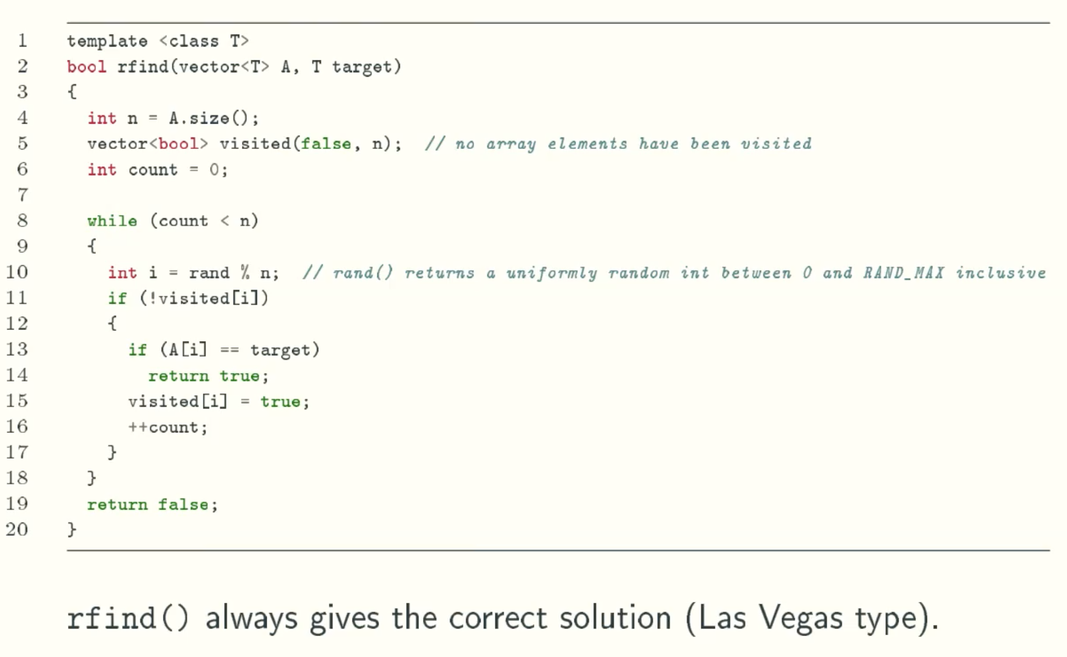
Solution Analysis

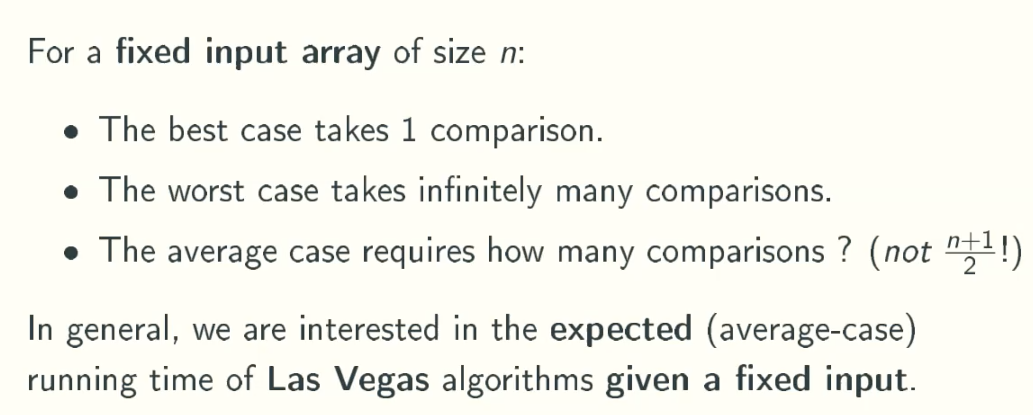
Average time

T is the iteration times
when target is in array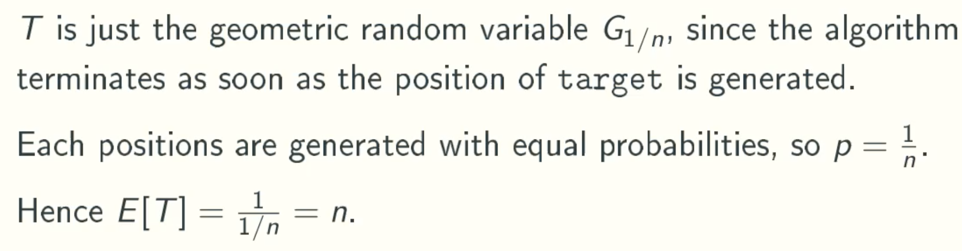

when target is not in array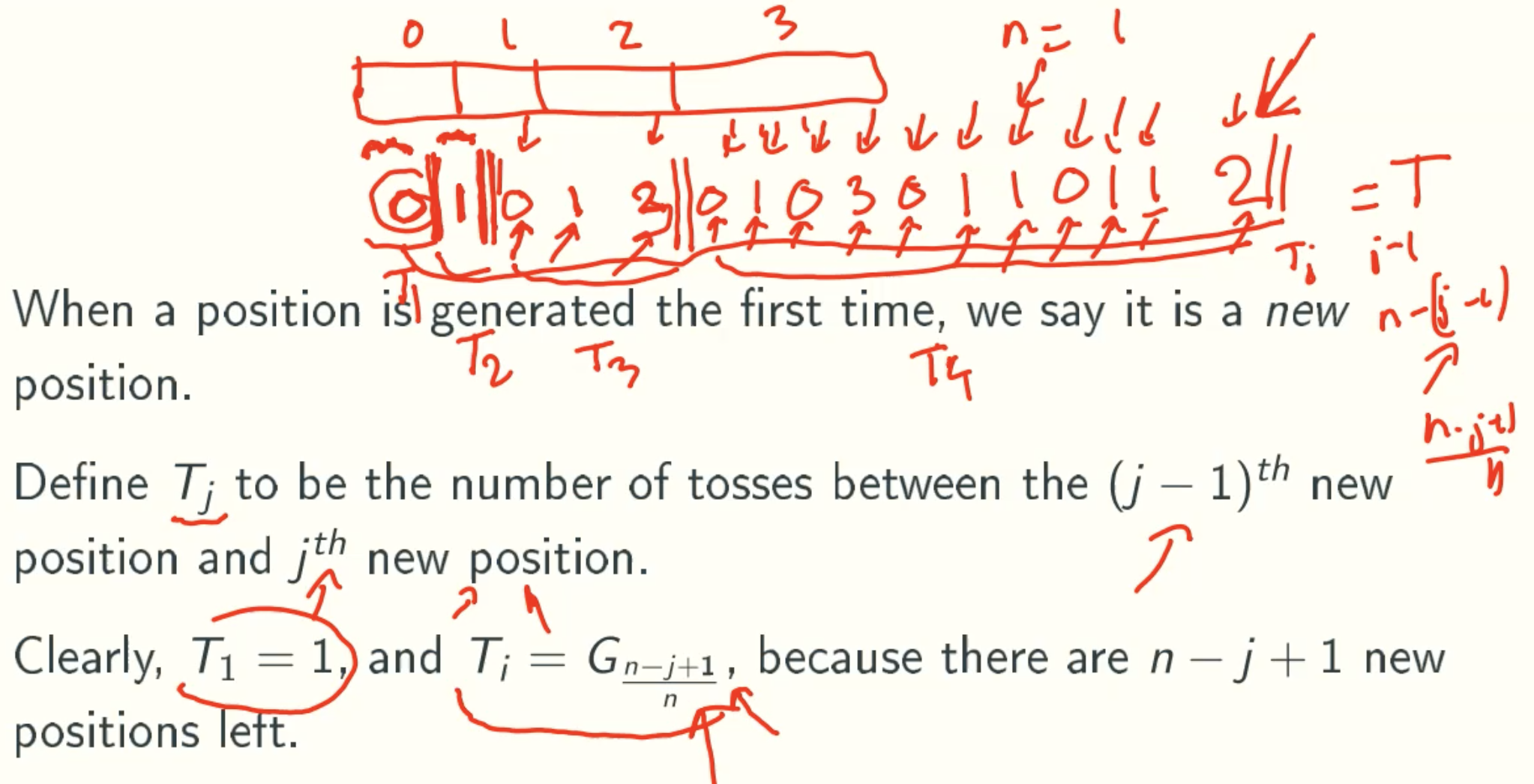

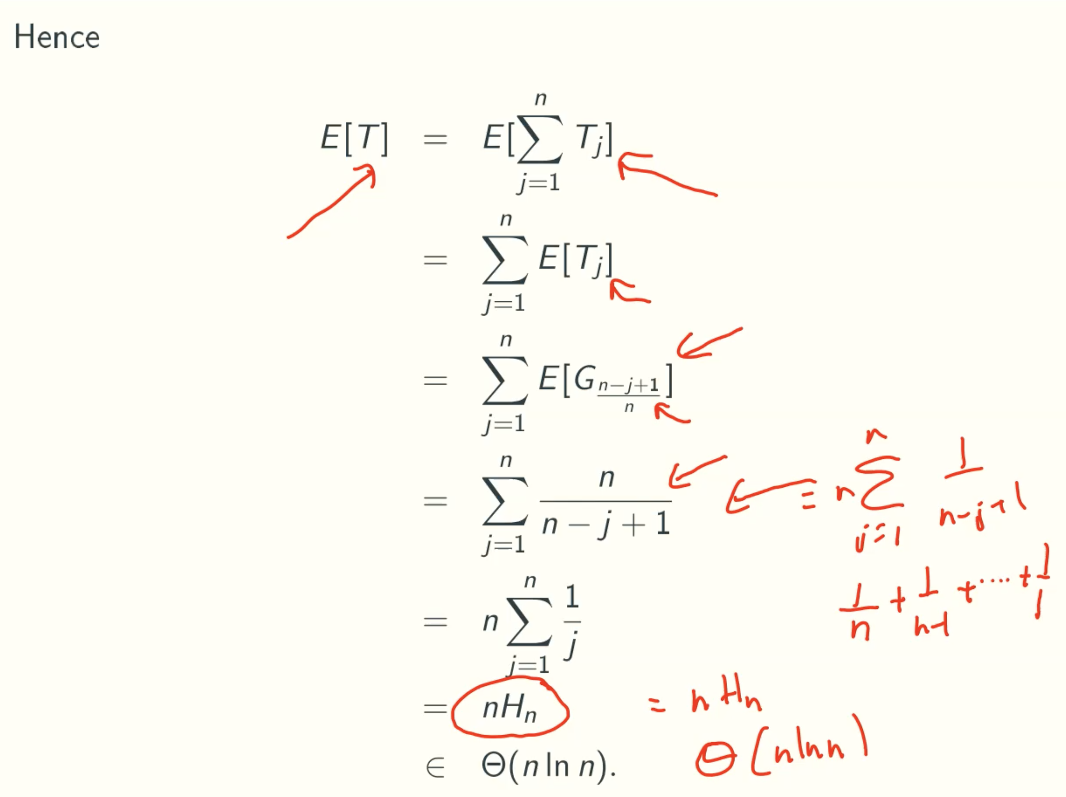
Example-Coupon Collection

Randomized Sorting

Problem defination

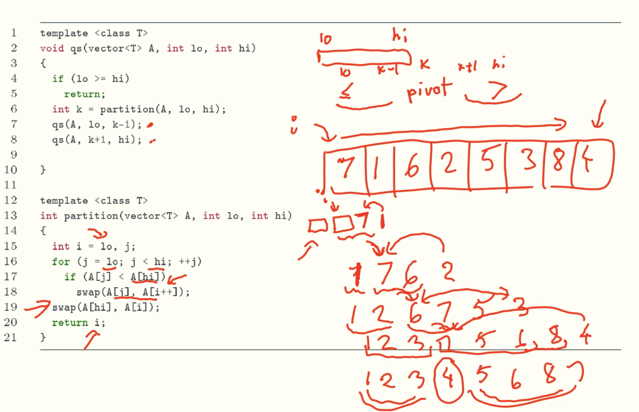
Deterministic Quicksort

Solution Analysis

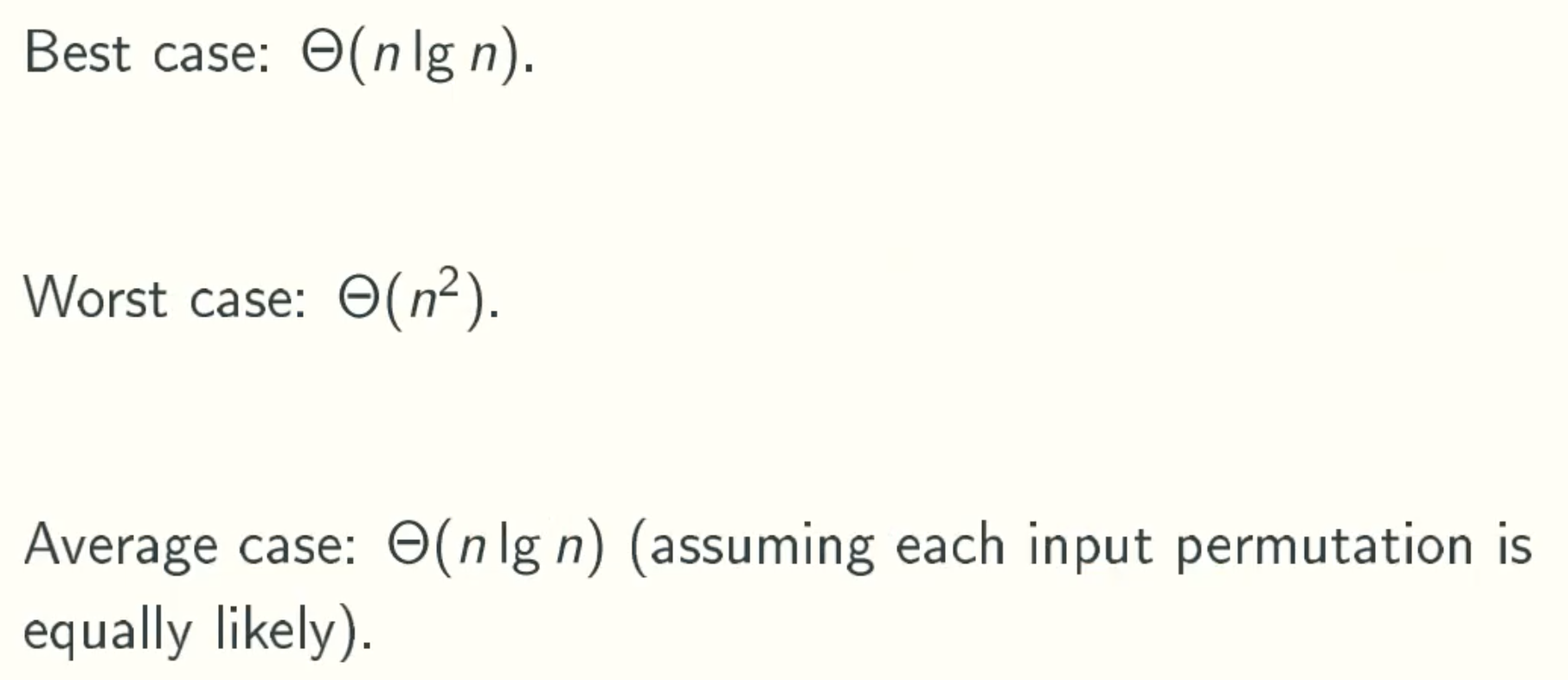
Average case
the partition are evenly, the depth of recursive tree is log(n) + 2

T（n）≤2T（n/2） +n，T（1）=0  (you need to compare all elements to find the right position of pivot)
T（n）≤2（2T（n/4）+n/2） +n=4T（n/4）+2n  
T（n）≤4（2T（n/8）+n/4） +2n=8T（n/8）+3n  
……  
T（n）≤nT（1）+（log2n）×n= O(nlogn)  (every level compare n times total, logn level compare nlogn times)

therefore, the running time is O(nlogn).

Worst case
the input array is totally ascending or descending, every partition just reduce one element, that is, its left or right is empty. So it need n iterations, and in each iteration the pivot needs to compare with all other elements. The running time is O(n²)

each input permutation is equally likely
the array is input randomly. Every input order has same probability.

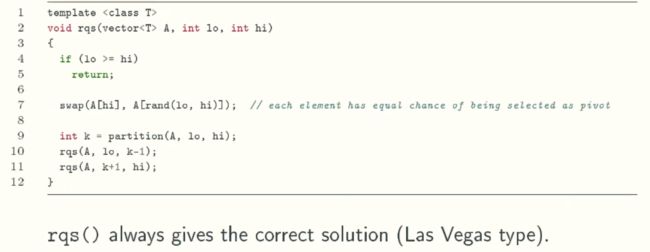
Randomized Quicksort

Expected running time analysis

Notation

For a fixed input array A[0..n-1]:

• Let C be the random variable counting the number comparisons made by randomized quicksort.
• Let a_i denote the i ^th smallest element of A[0..n-1], a_i is not the element at position i.

When is C_i,j is 1?

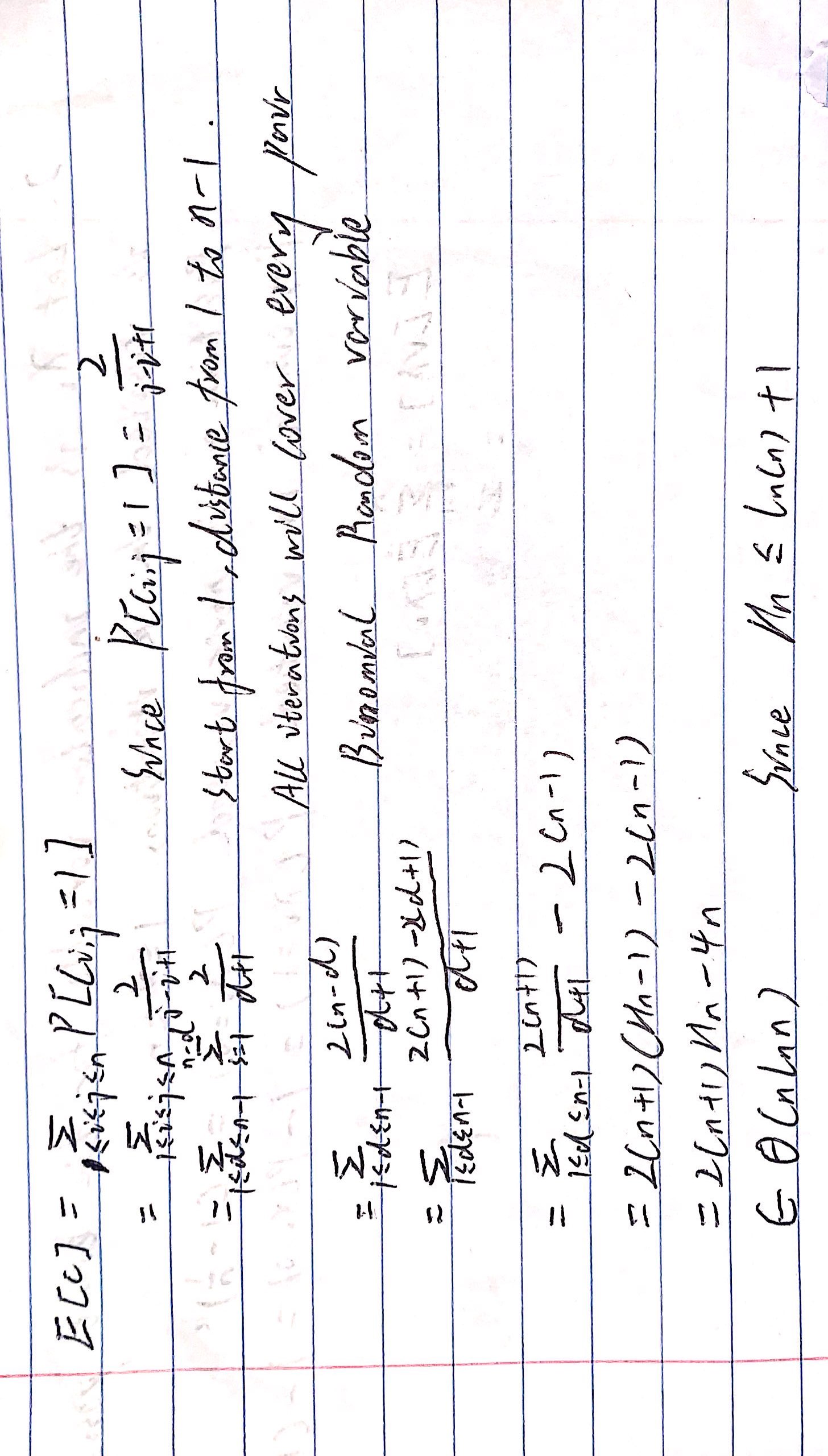
P(C_i,j = 1) = 2/(j-i+1)
since there are j - i + 1 elements in a_i…a_j. C_i,j == 1 when C_i or C_j is pivot,. And each element has the same probability to become pivot, therefore, P(C_i,j == 1) = 2/(j-i+1).

Using linearity of expection to compute E[C]

Randomized Selection

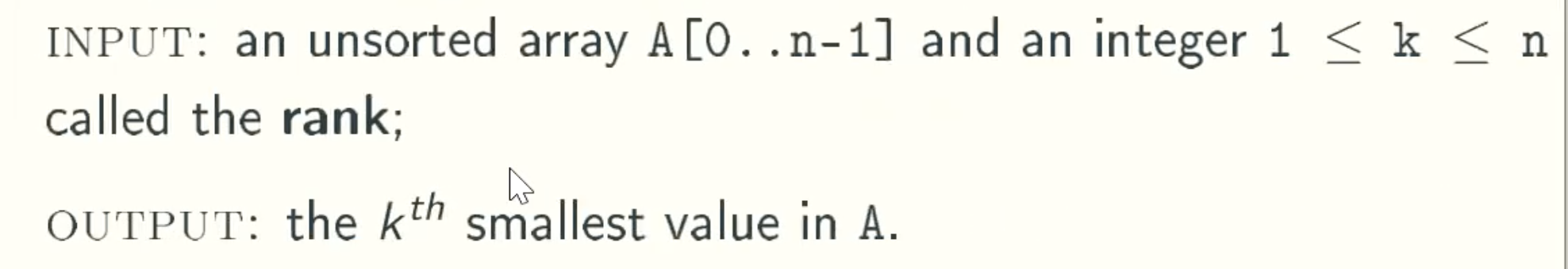
Problem defination

Deterministic QuickSelect

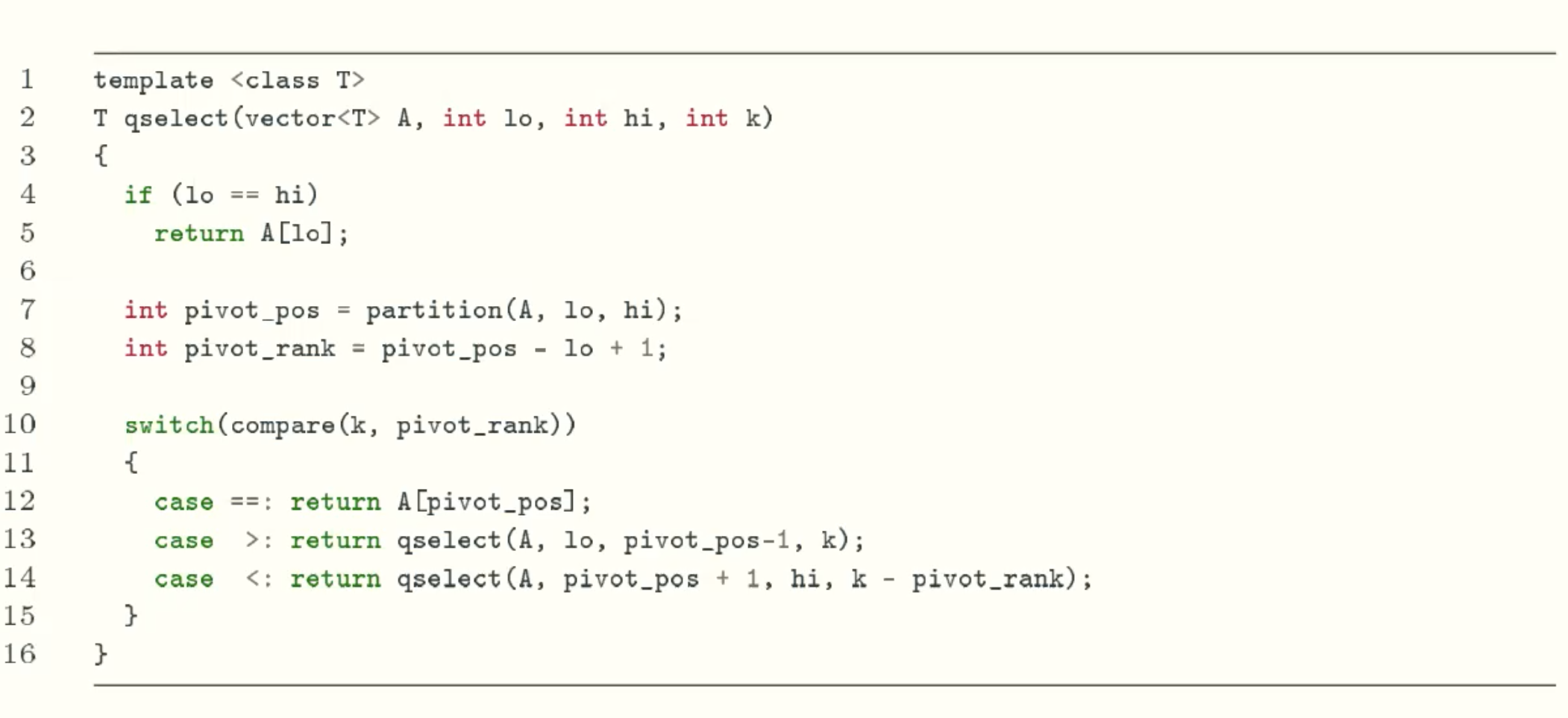
Solution Analysis

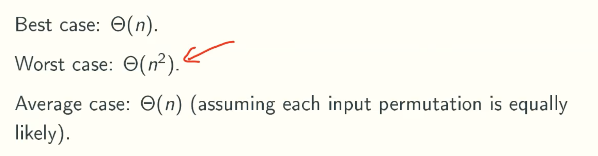
Randomized QuickSelect

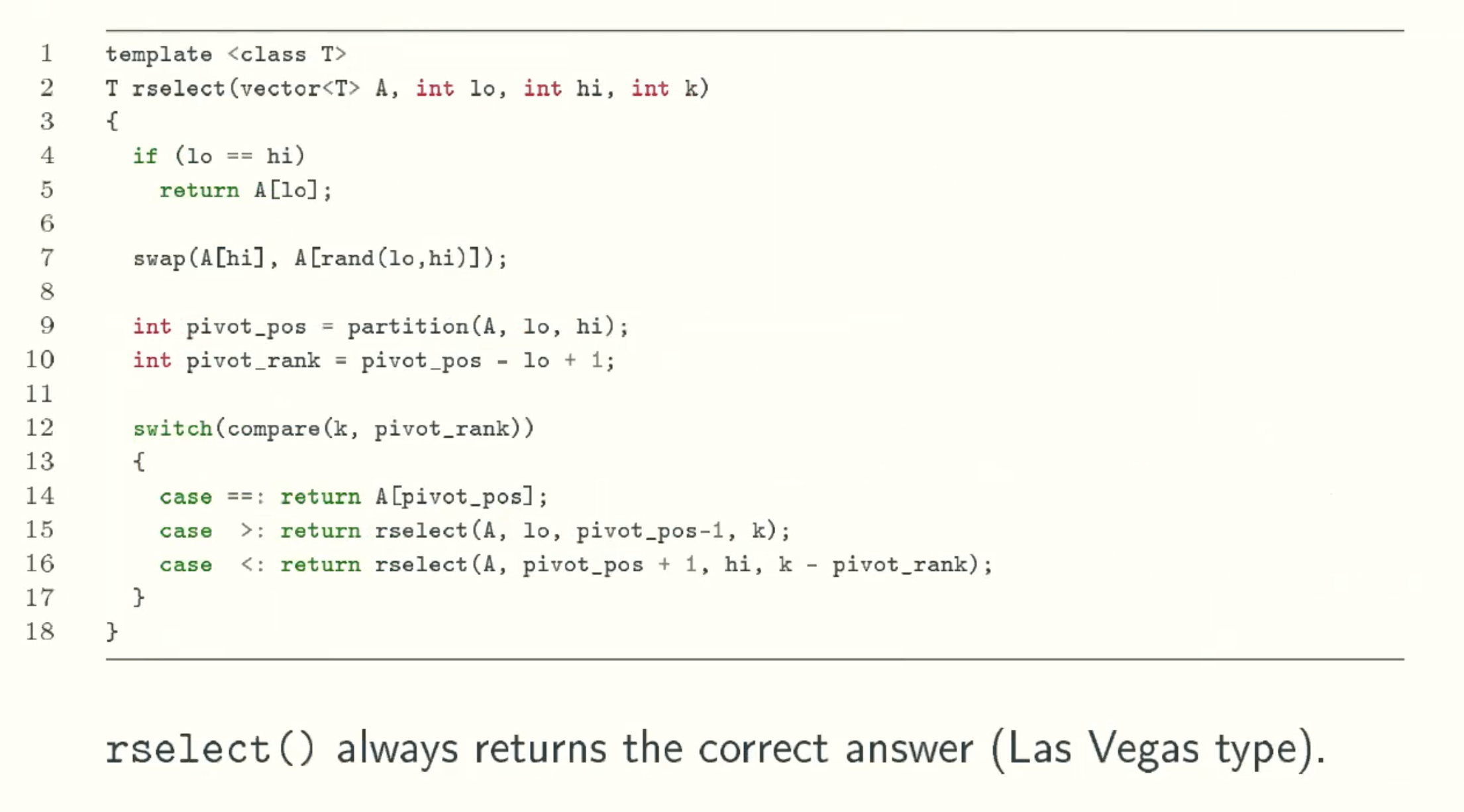
Solution Analysis

Assumption:
For a fixed input array A of size n and a fixed rank k
Let C be the random variable counting the number of comparisons.
Let a_i be the i^th smallest value in A.
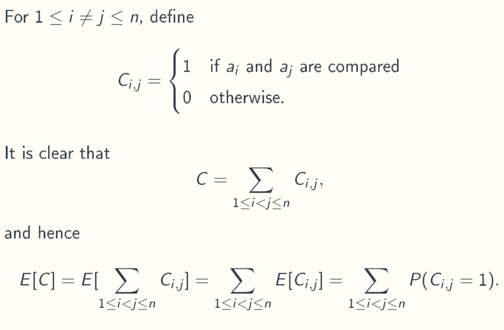
C = ∑_1<=i<=j<=nC_i,j, where
C_i = 1 if a_i and a_j is compared
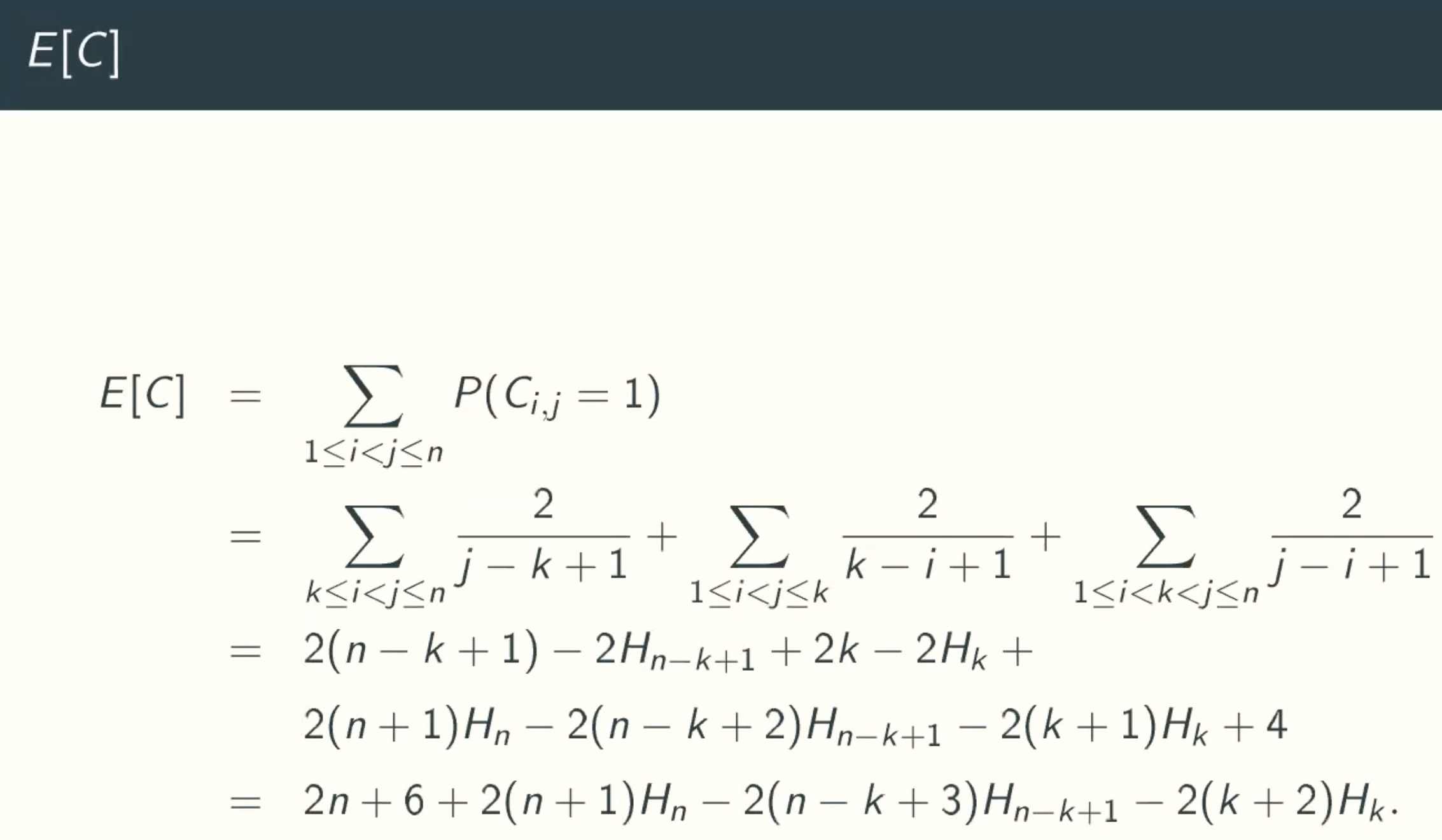
E[C] = E[∑_1<=i<=j<=nC_i,j] = ∑E[C_i,j] = ∑P(C_i,j = 1)

when C_i,j = 1?

i is always less than j

1. k <= i < j
   Let a_p be the next pivot:
   • p < k or p > j, a_i and a_j and k will belong to the same partition.
   • k <= p < i, a_i and a_j will never be compared, C_i,j = 0.
   • i < p < j, a_i and a_j will belong to different partition, they will never be compared, C_i,j = 0.
   • p = i or p = j, pivot will be compared with every other elements, C_i,j = 1.

Since each element in the set(a_k, a_k+1, a_k+2, …… a_j) has equal chance of being selected as the pivot.
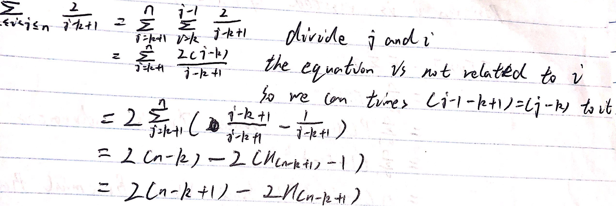
P(C_i,j=1) = 2 / (j-k+1)

summing over all k <=i < j <= n

2. i < j <= k
   Let a_p be the next pivot:
   • p < i or p > k, a_i and a_j and k will belong to the same partition.
   • j < p <= k, a_i and a_j are discarded and C_i,j = 0.
   • i < p < j: a_i and a_j will never be compared and C_i,j = 0.
   • p = i or p = j, C_i,j = 1.

Since each element in the set(a_i, a_i+1, a_i+2, …… a_k) has equal chance of being selected as the pivot.
P(C_i,j=1) = 2 / (k-i+1)

summing over all 1 <=i < j <= k

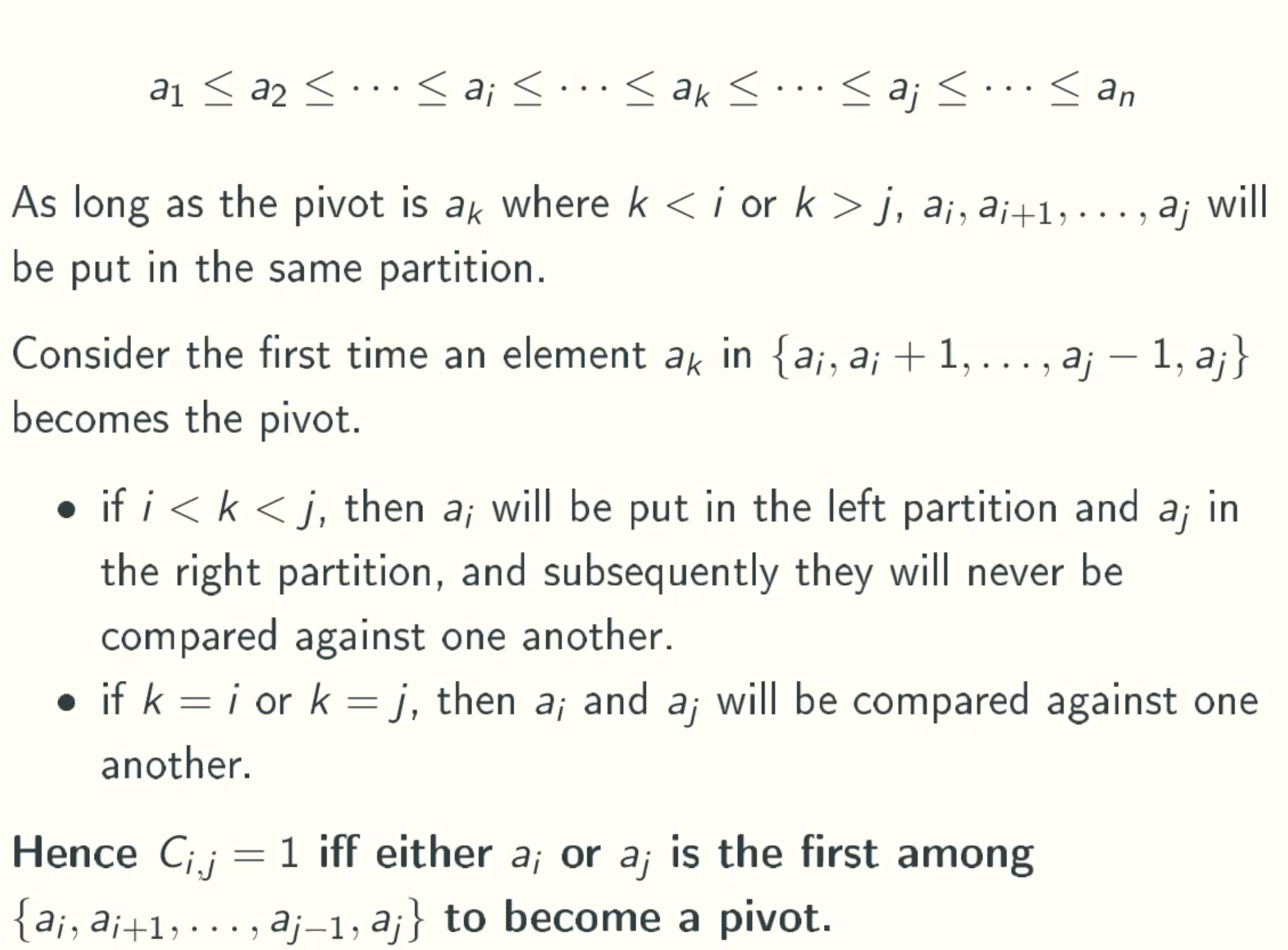
3. i < k < j
   Let a_p be the next pivot:
   • p < i or p > j, a_i and a_j and k will belong to the same partition.
   • i < p < j, a_i and a_j will never be compared, C_i,j = 0.
   • p = i or p = j, C_i,j = 1.

Since each element in the set(a_i, a_i+1, a_i+2, …… a_j) has equal chance of being selected as the pivot.
P(C_i,j=1) = 2 / (j-i+1)

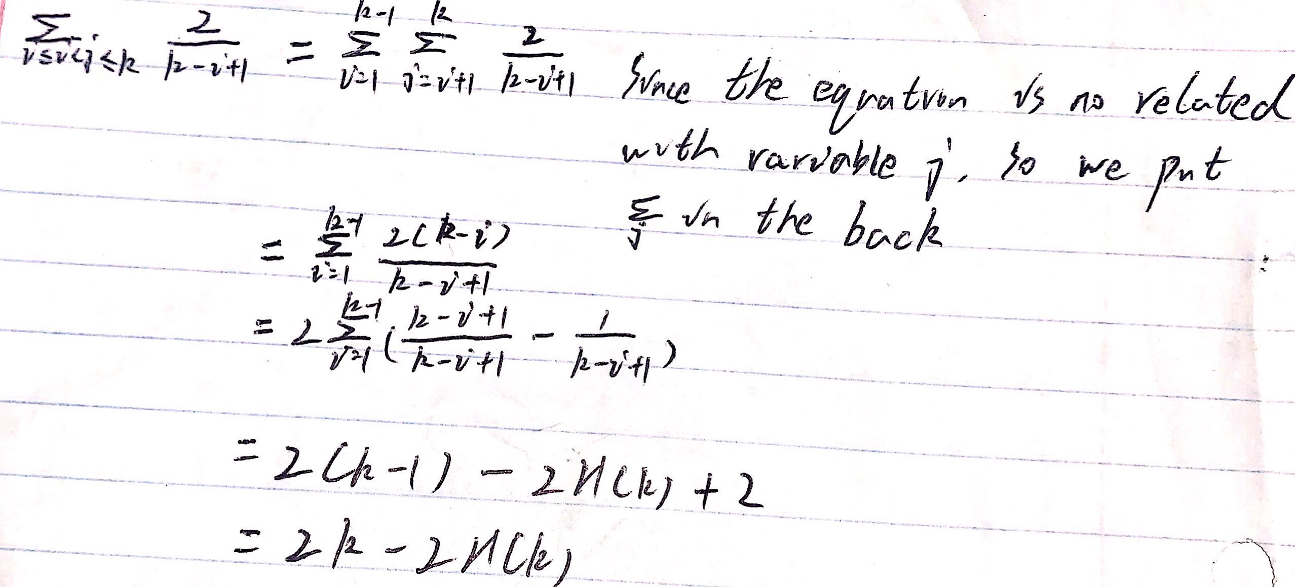
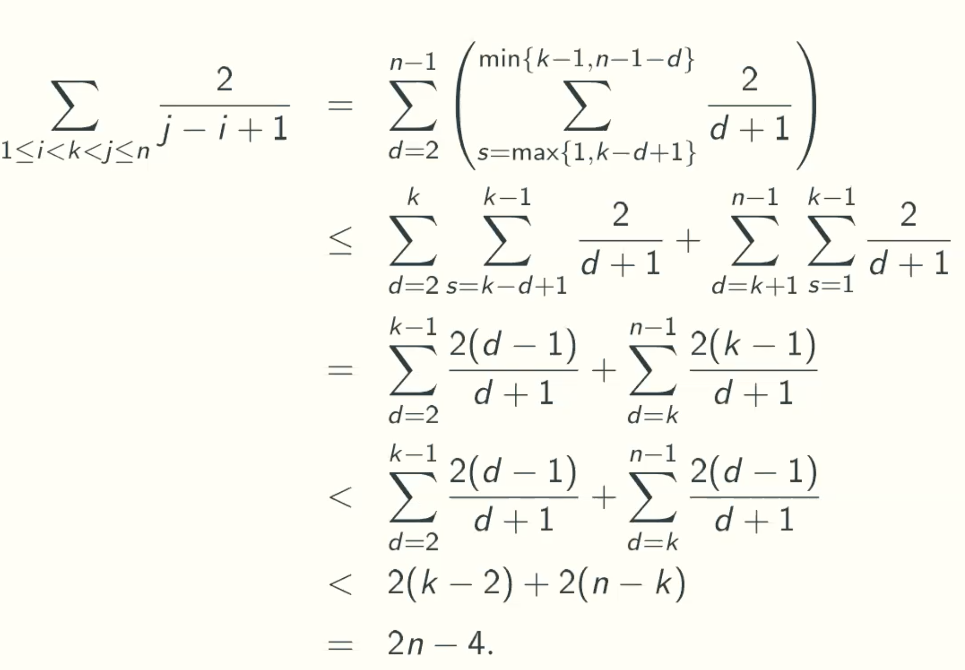
summing over all 1 <= i < k < j <= n

Q&A:

1. why the range of s is from max{1, k-d+1} to min{k-1, n-1-d}?
   s is from max{1, k-d+1}. Because the minimize distance between k and j is 1, the distance between i and j is d, therefore the distance between i and k is max (k-(d-1)) = k-d+1. At the same time, the start must be positive. So the start is from max{1, k-d+1}.
   s is to {k-1, n-1-d}. Because the maximize j is n-1, and the distance between i and j is d, therefore, the maximize i(start) is n-1-d. At the same time, i is smaller than k. So the start is to min{k-1, n-1-d}.

2. What is the purpose of the segmentation in second row?
   Divide d into two parts according to whether it is greater than k.
   In the first part, because d is smaller or equal to k, therefore k-d+1 must be postive, and i(start) must smaller than k, therefore the range is from k-d+1 to k-1.
   In the second part, because d is larger than k, therefore k-d+1 must be negative, so we choose 1 be the start, and from the same reason the maximize start is k-1, so the range is from 1 to k-1.

3. Why we can change k to d directly in row 3 to row 4?
   In the second part, d is bigger than k. So if the fourth row is less than the third row, we can just replace k with d.

4. Why ∑(2(d-1)/(d+1))+∑(2(d-1)/(d+1)) < 2(k-2)+2(n-k)?
   

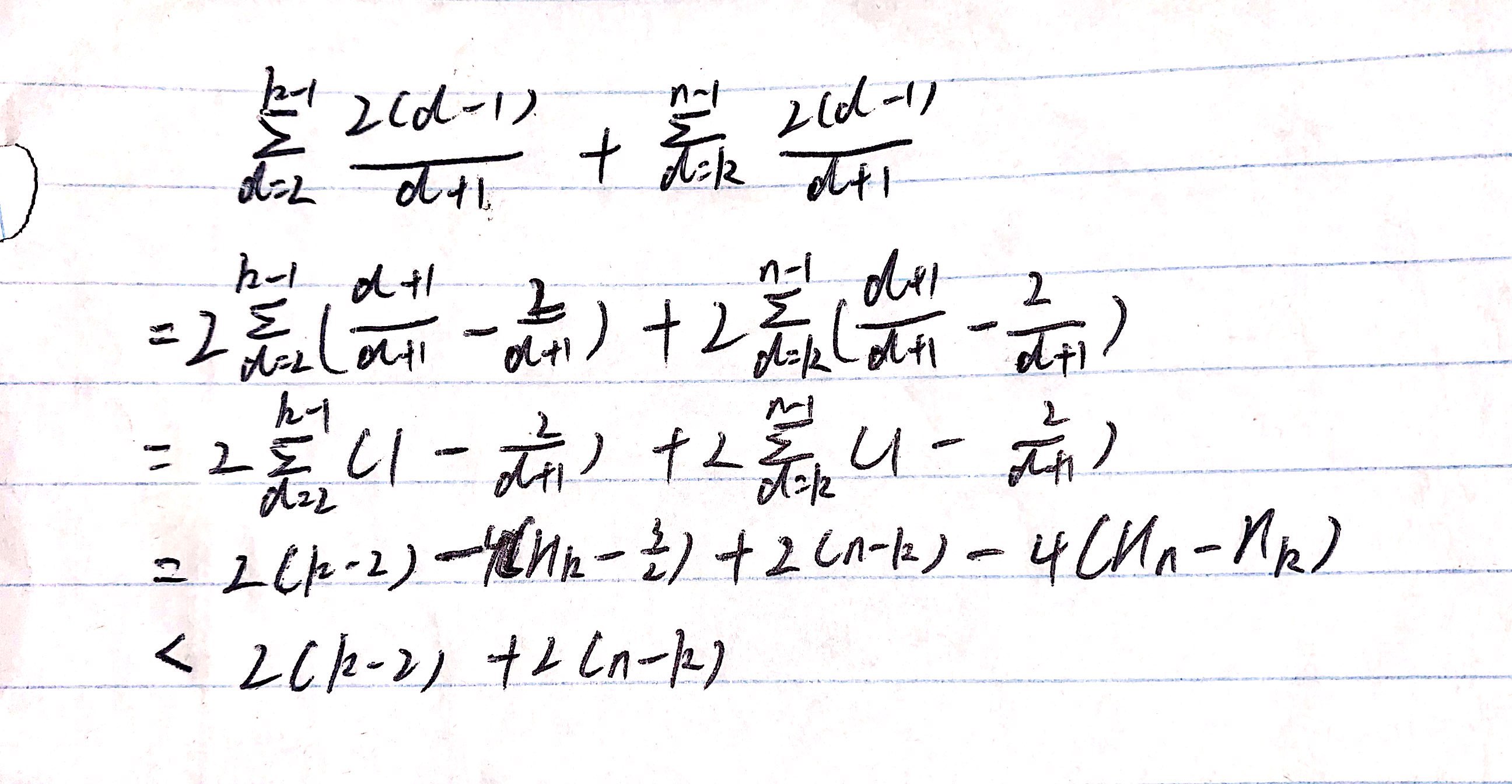
E[C] < θ(n)

adding all situations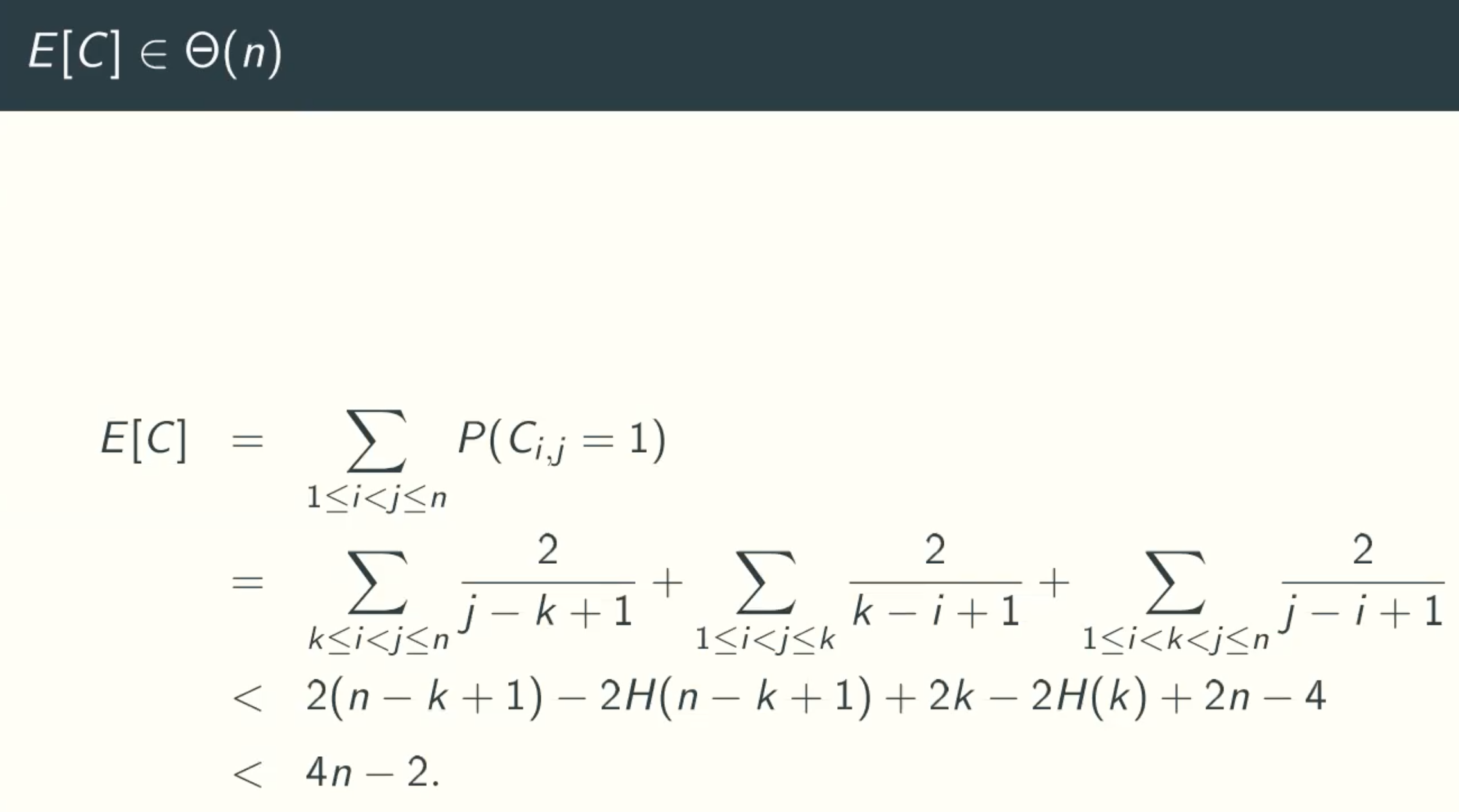

Esxactly Formula Of E[C]

Primality Testing

Problem Defination

Upper Bound

Randomized Solution:Fermat test

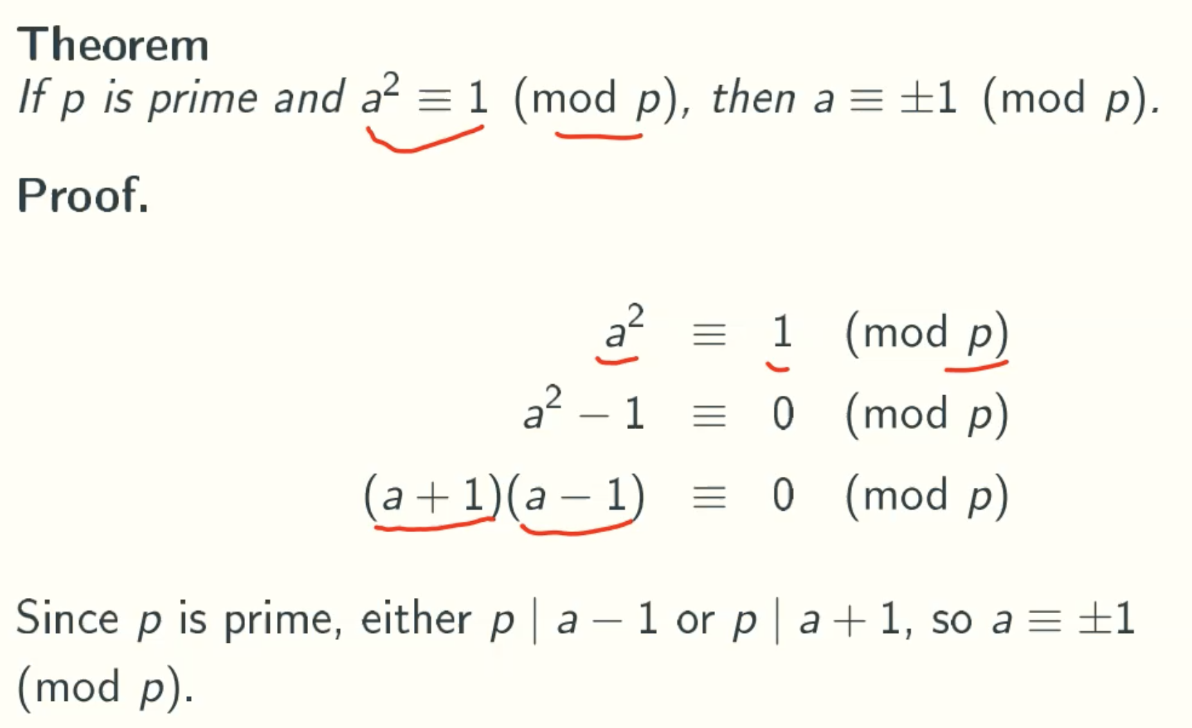
Theorem

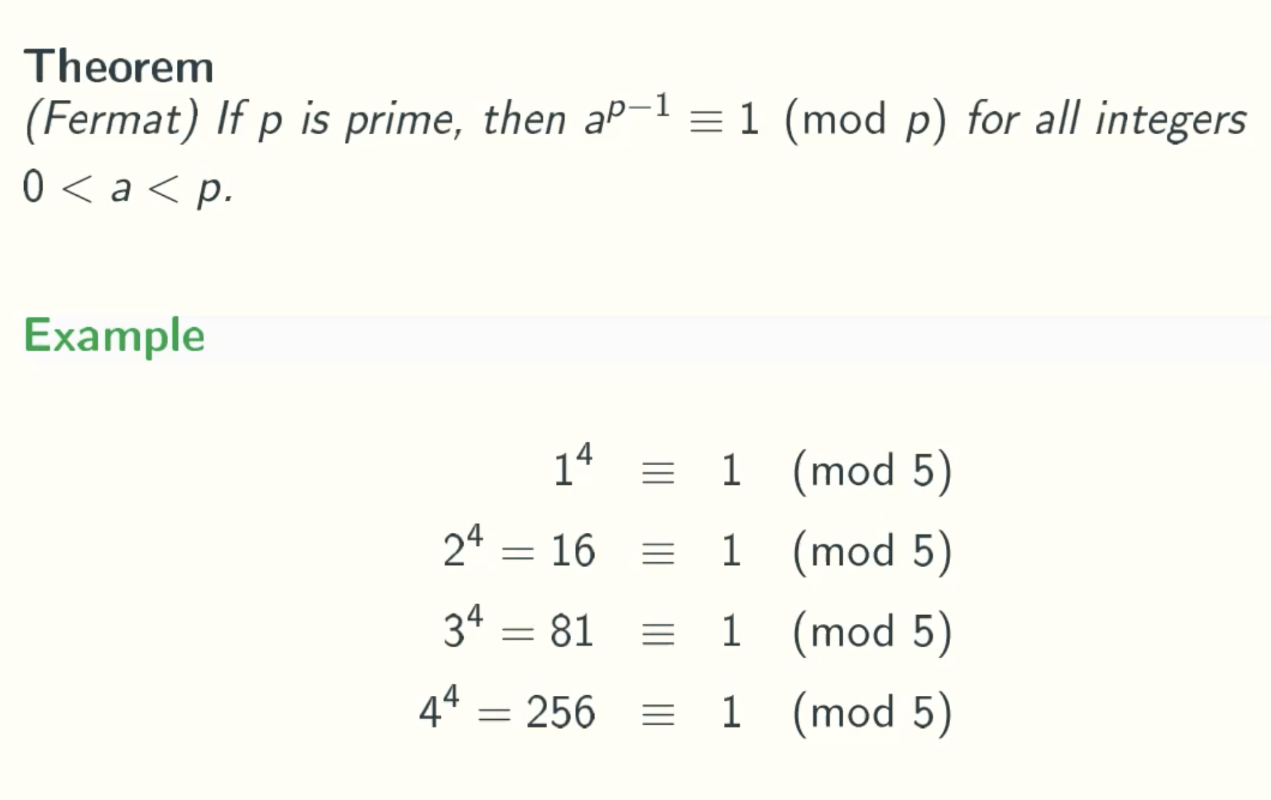
Theorem Proof

Q&A

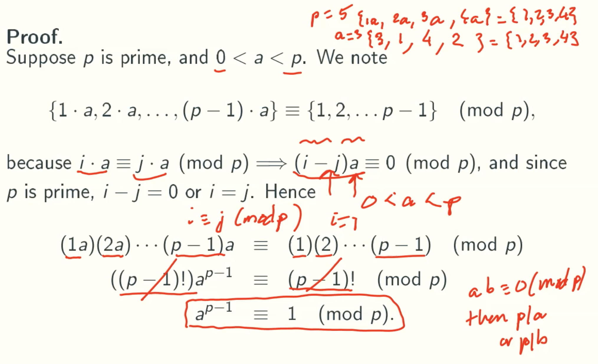
1. Why {1a, 2a, 3a, … (p-1)a} = {1, 2, 3, …, p-1} mod p?
   For any prime p and any a smaller than p, the left is the same set with right.
   For example p = 5, a = 3.
   left={1,2,3,4}, right = {3,1,4,2}.
2. What does that mean if ab = 0 (mod p)?
   it means p%a = 0 or p%b = 0.
3. Why (1a)(2a)…(p-1)a = ((1)(2)…(p-1))(mod p)?
   Since the left and right is the same set, so the product of all elements is equal. That is, the product of {1,2,3,4} is equal to the product of {3,1,4,2}.

New Idea

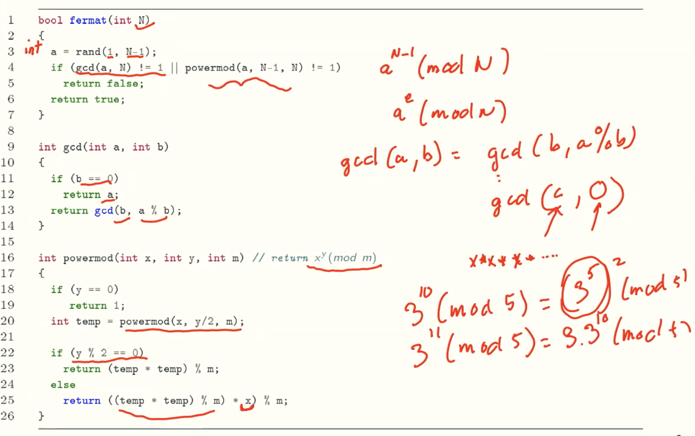
Implementation

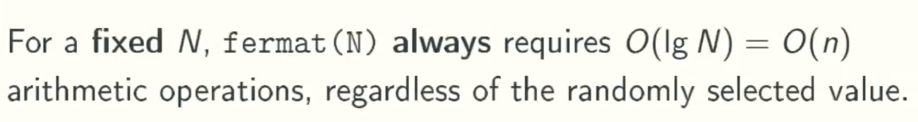
Error Situation

When N is 3*5 = 15, the a is 4, the answer is incorrect.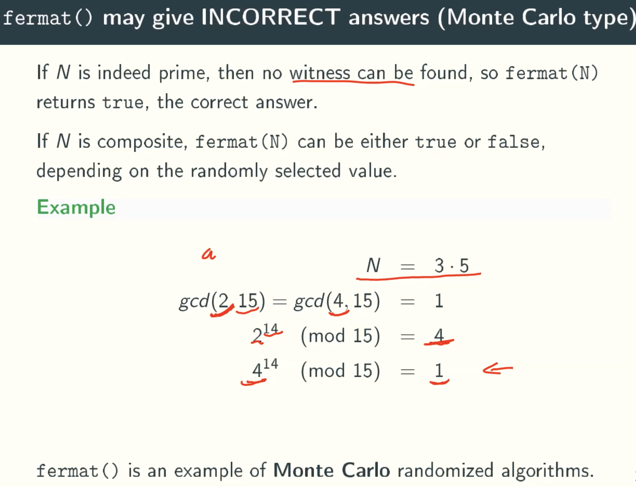

Error Probability

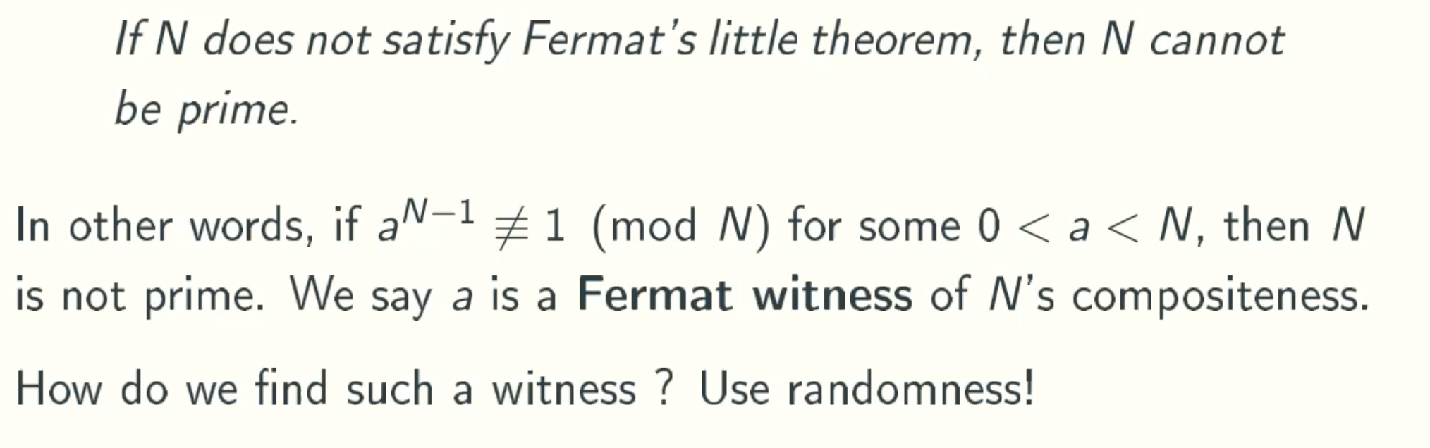
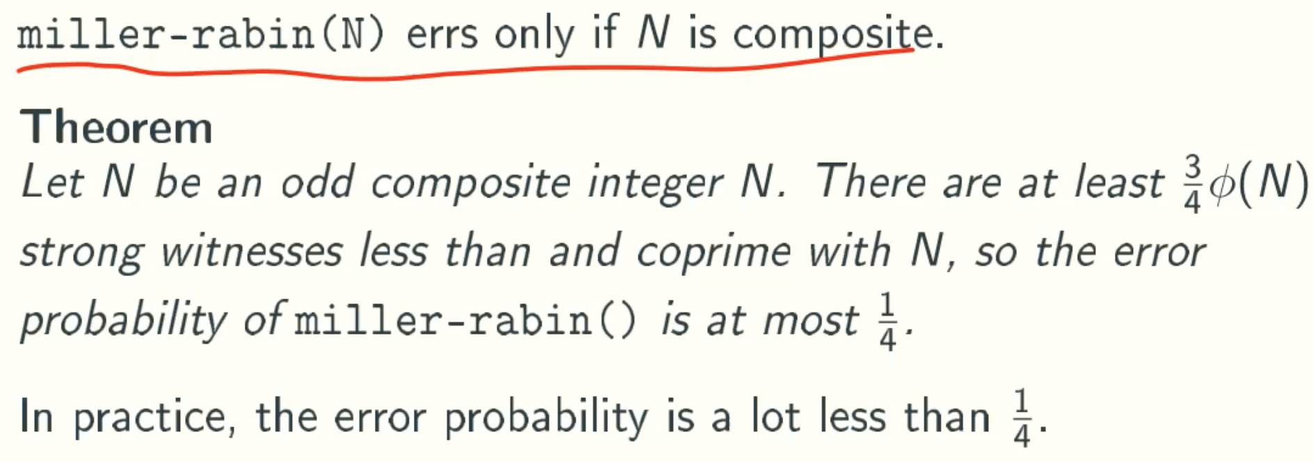
fermat(N) errors only if N is composite.
ϕ(N) = {0<a<N, gcd(a,N)=1}

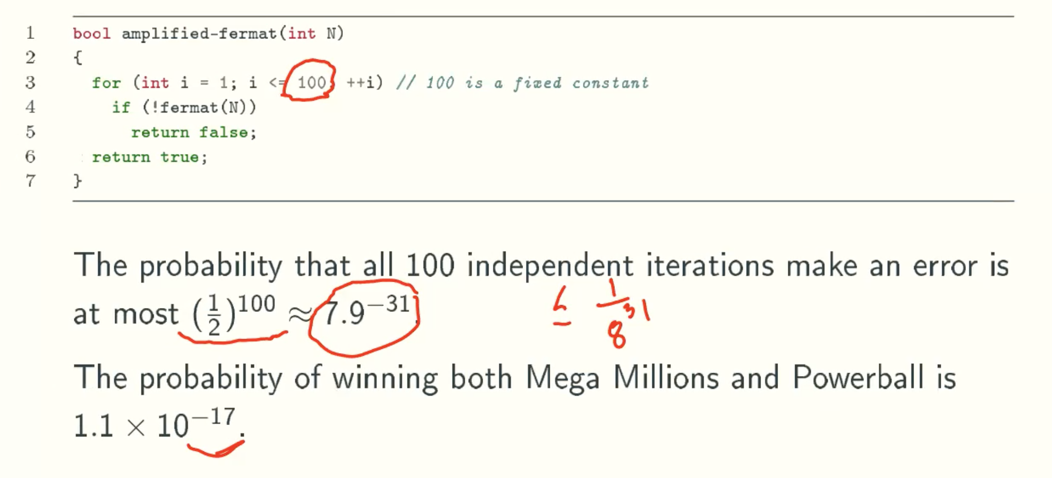
• If N has one Fermat witness a that it is composite, then there must be a lot witnesses they are composited and the error probablity is at most 1/2.
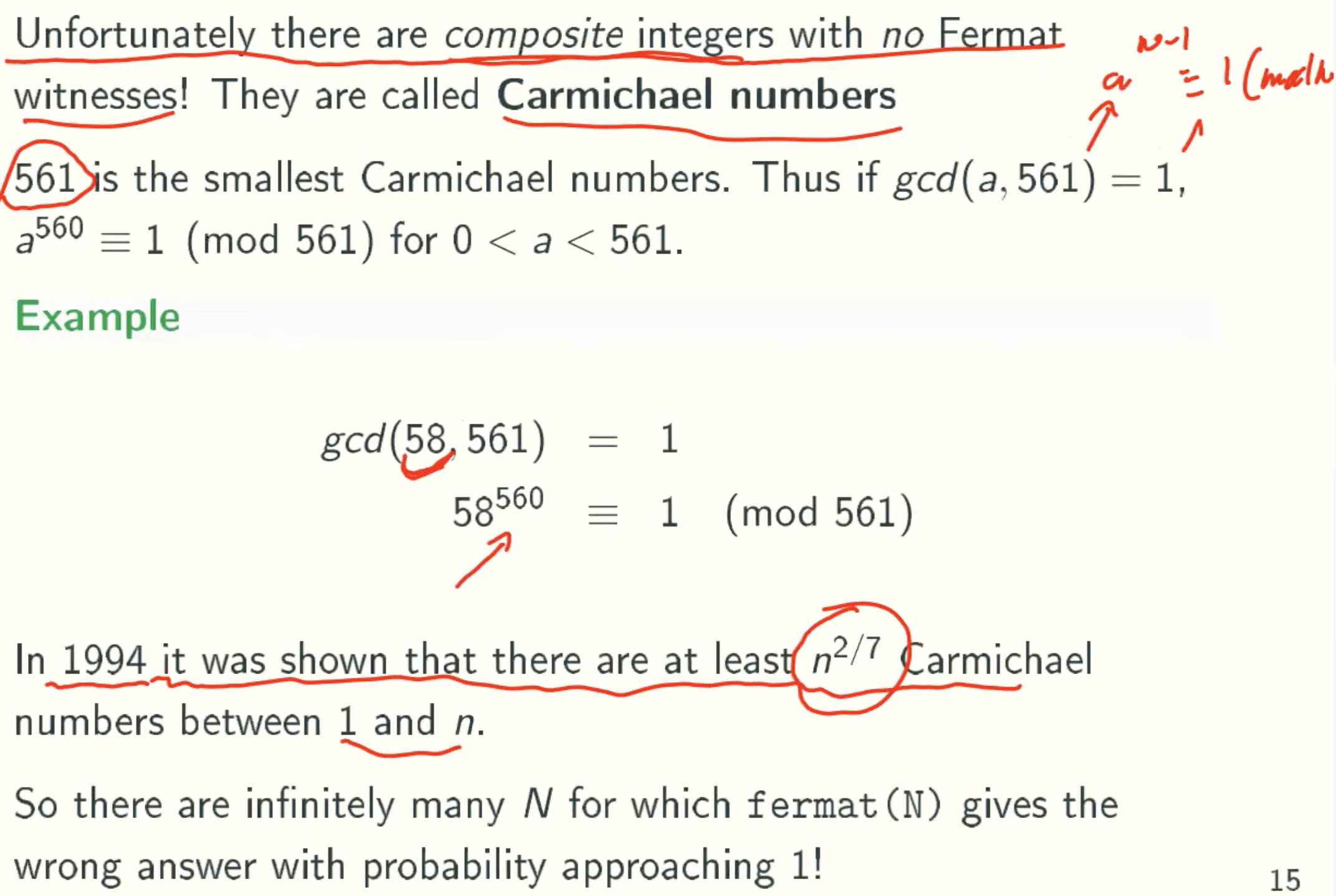
  That is because If there is one witness a and other nonwitness set {b₁, b₂, b₂, b₃, …}, there must be a witness set {ab₁, ab₂, ab₂, ab₃, …}, So there are at least 1/2 witness, the error probability at most is 1/2.
• If N has no Fermat witness, then the error rate is at least ϕ(N)/N -> 1/N -> ∞, where ϕ(N) is the number of positive integers smaller than and coprime with N.

Reduce Error Probability from 1/2 to insignificant

Carmichael numbers

Randomized Solution:Miller-Rabin

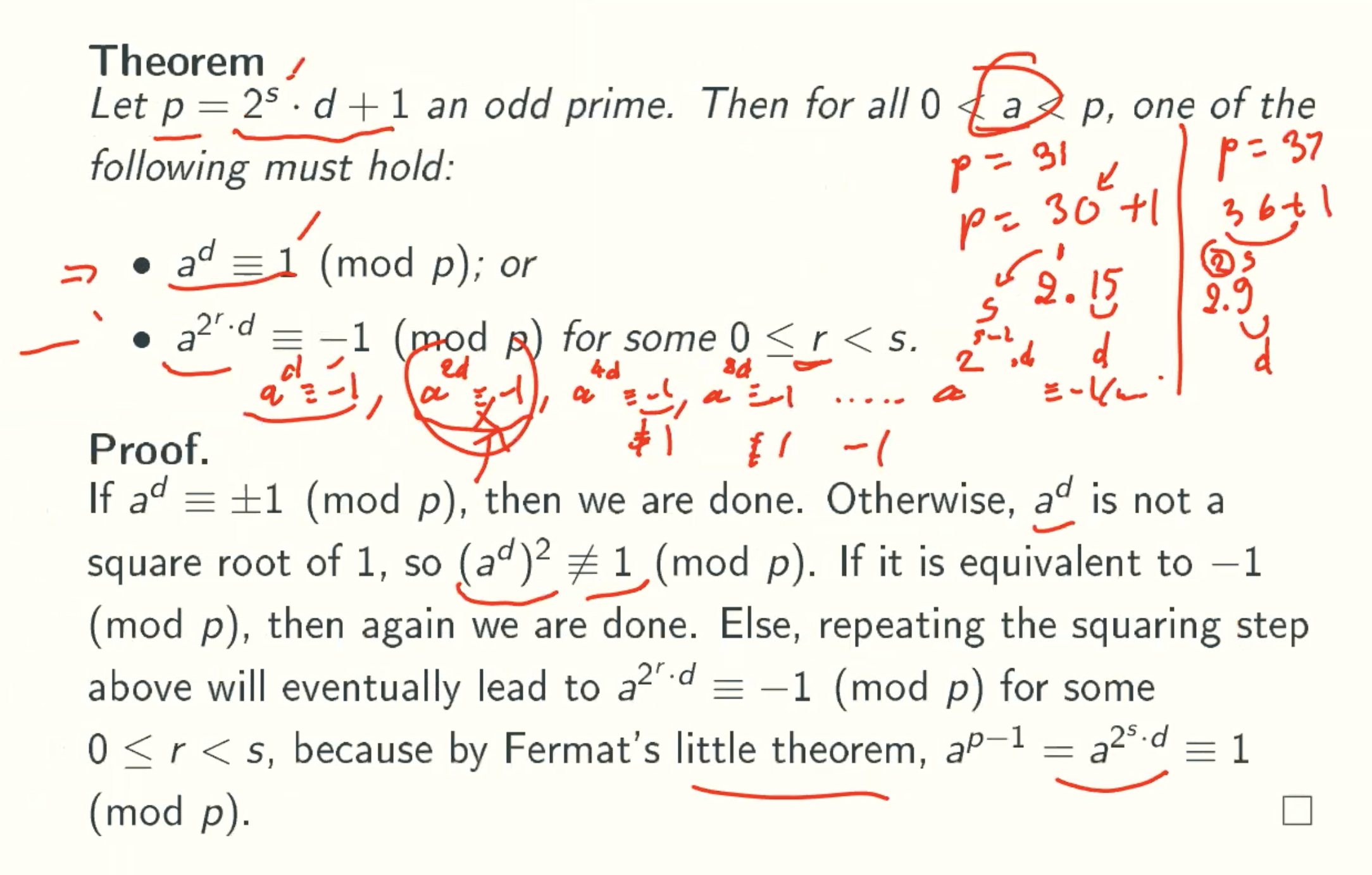
Theorem

Modified Theorem

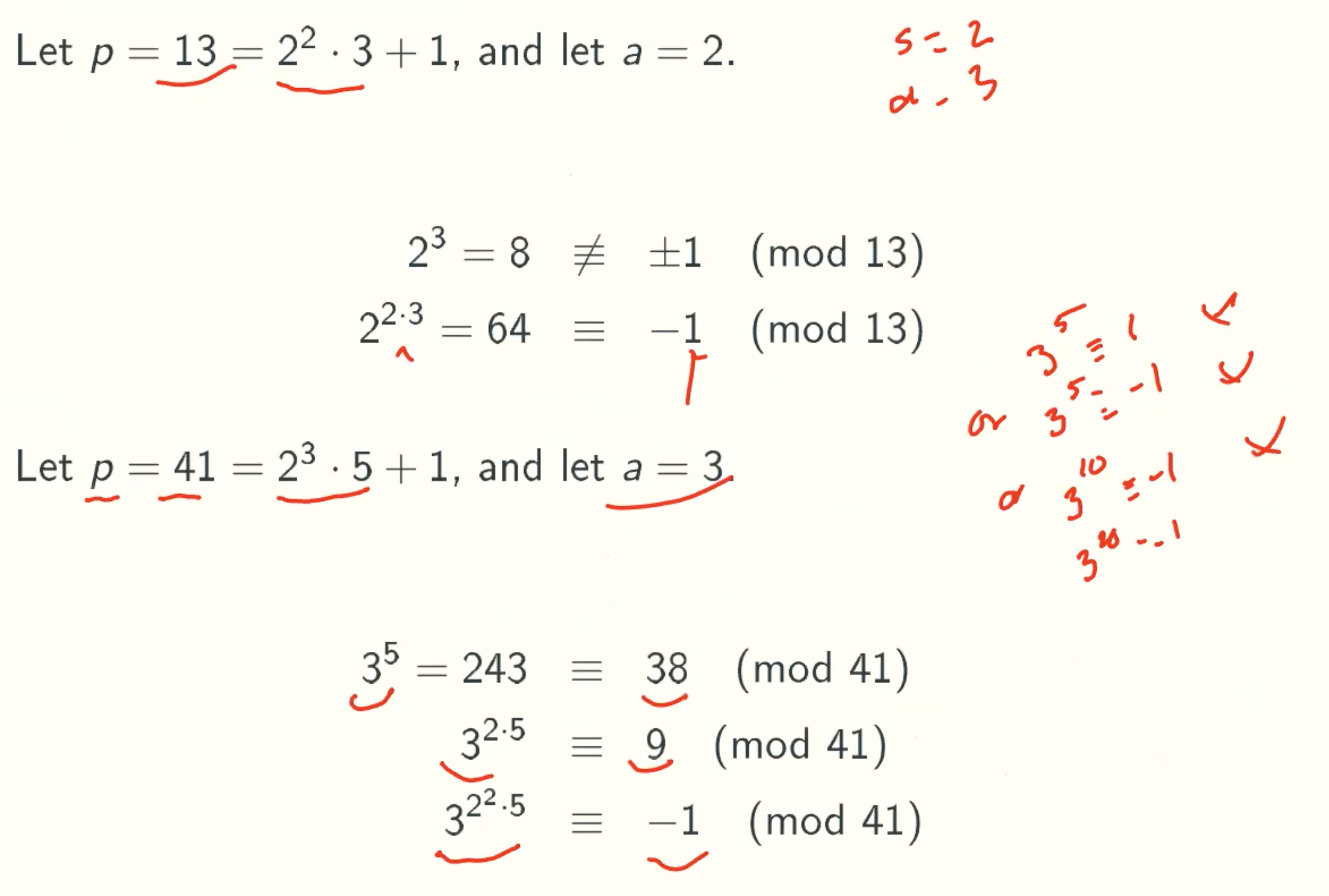
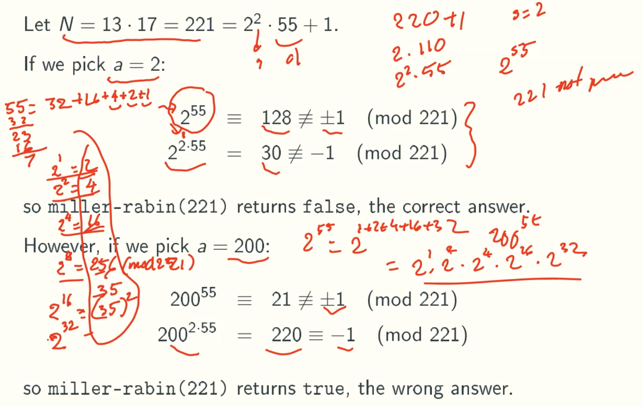
Example

Implementation Idea

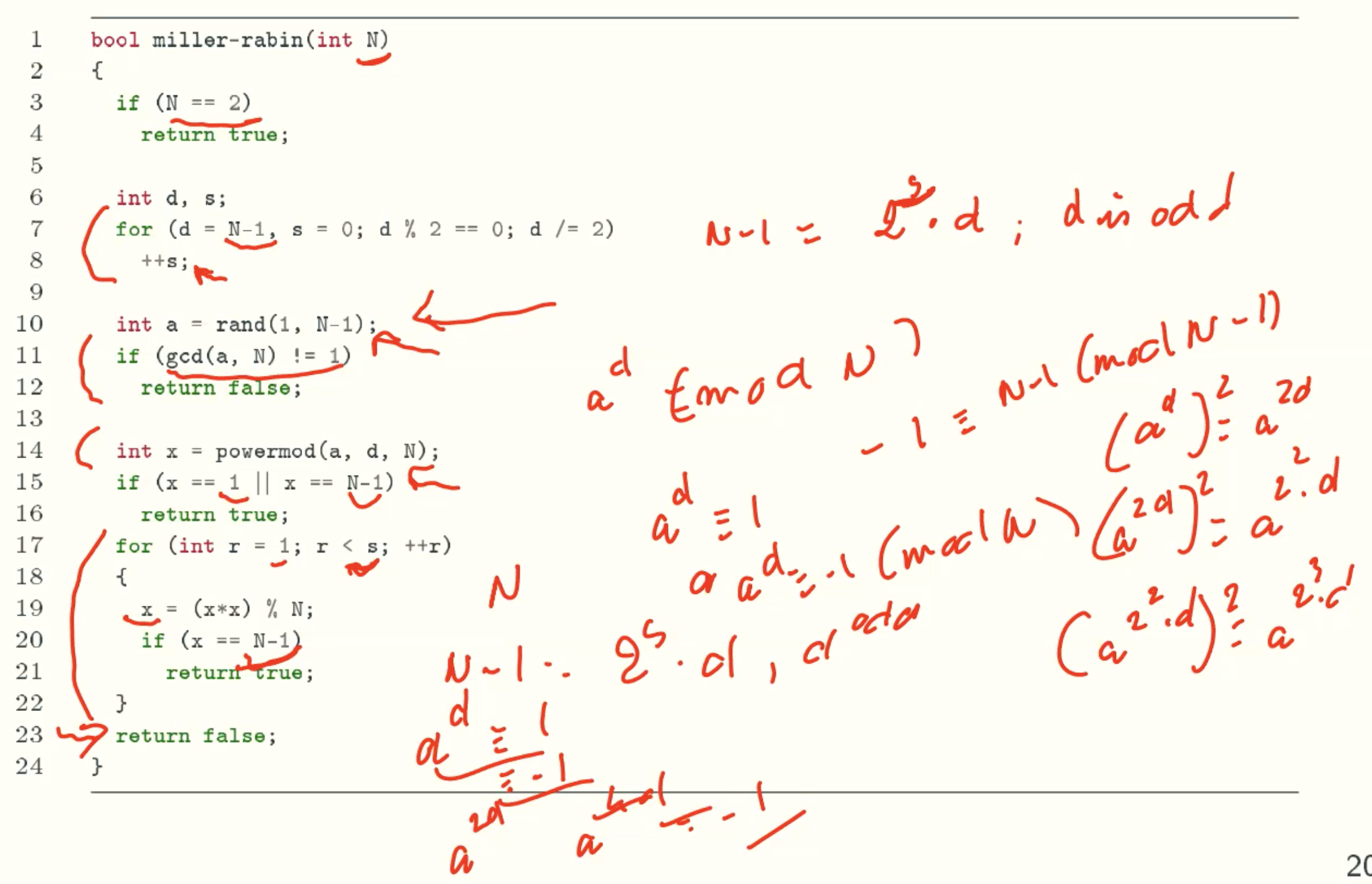
Q&A

1. Why N-1 == -1?

-1 = (N-1) mode (N). Like 64 = -1 (mod 13) = 12 (mod 13)
Since mod just return positive result in C++, so we choose N-1 here.

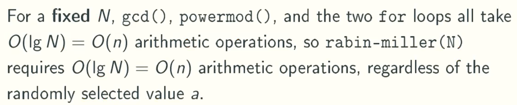
Solution Analysis

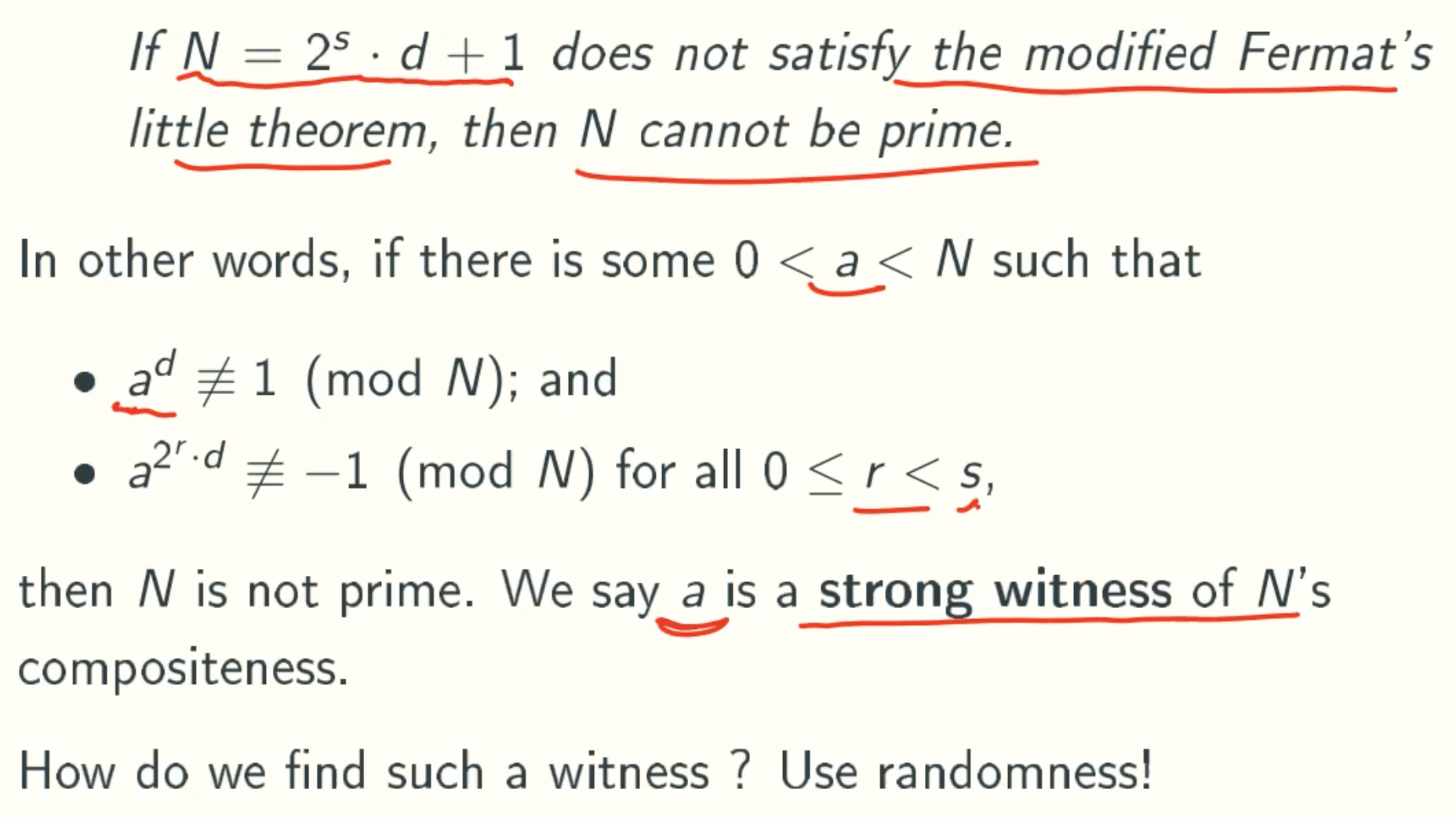
Error Situation

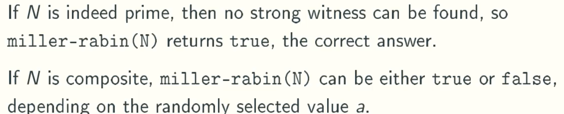
Error Probability

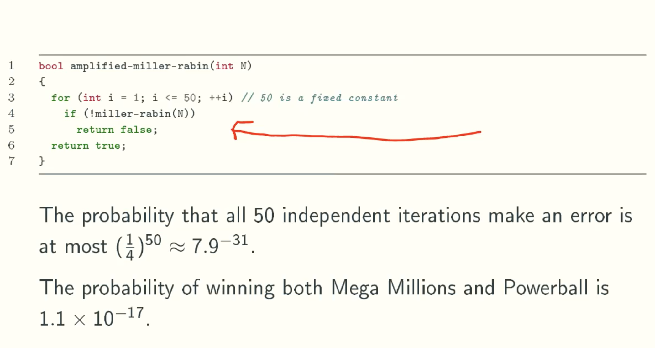
Reduce Error Probability from 1/4 to insignificant

Amortized Analysis

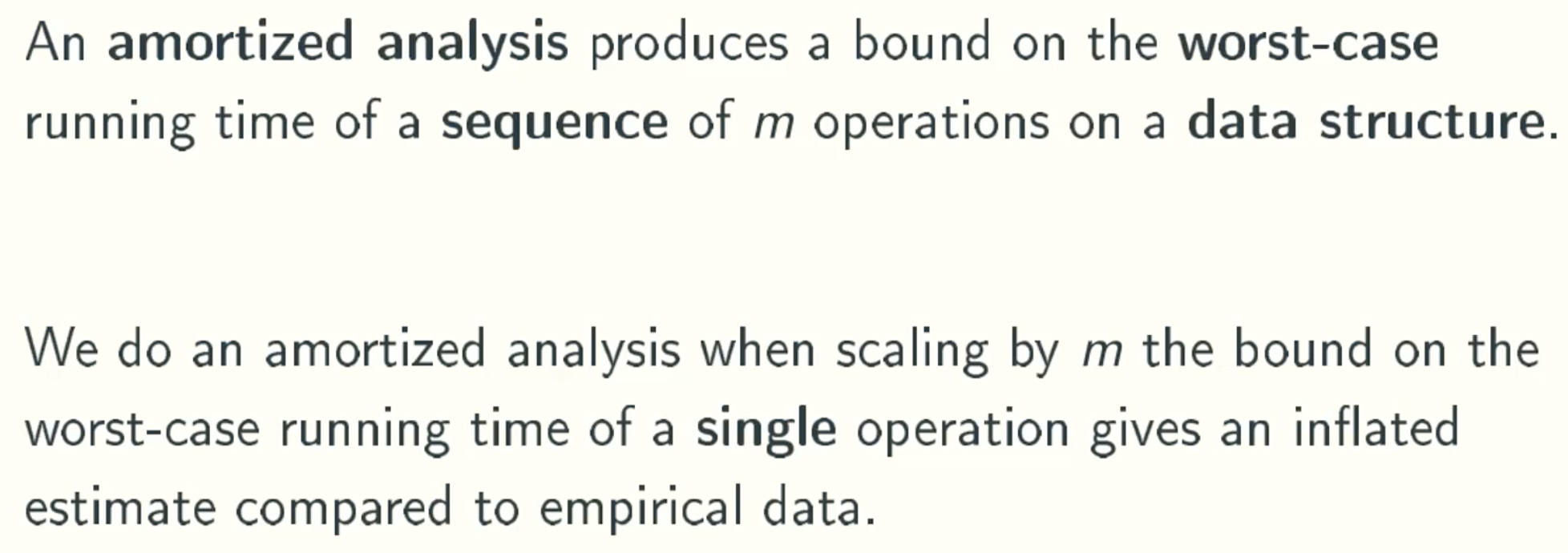
What Is Amortized Analysis

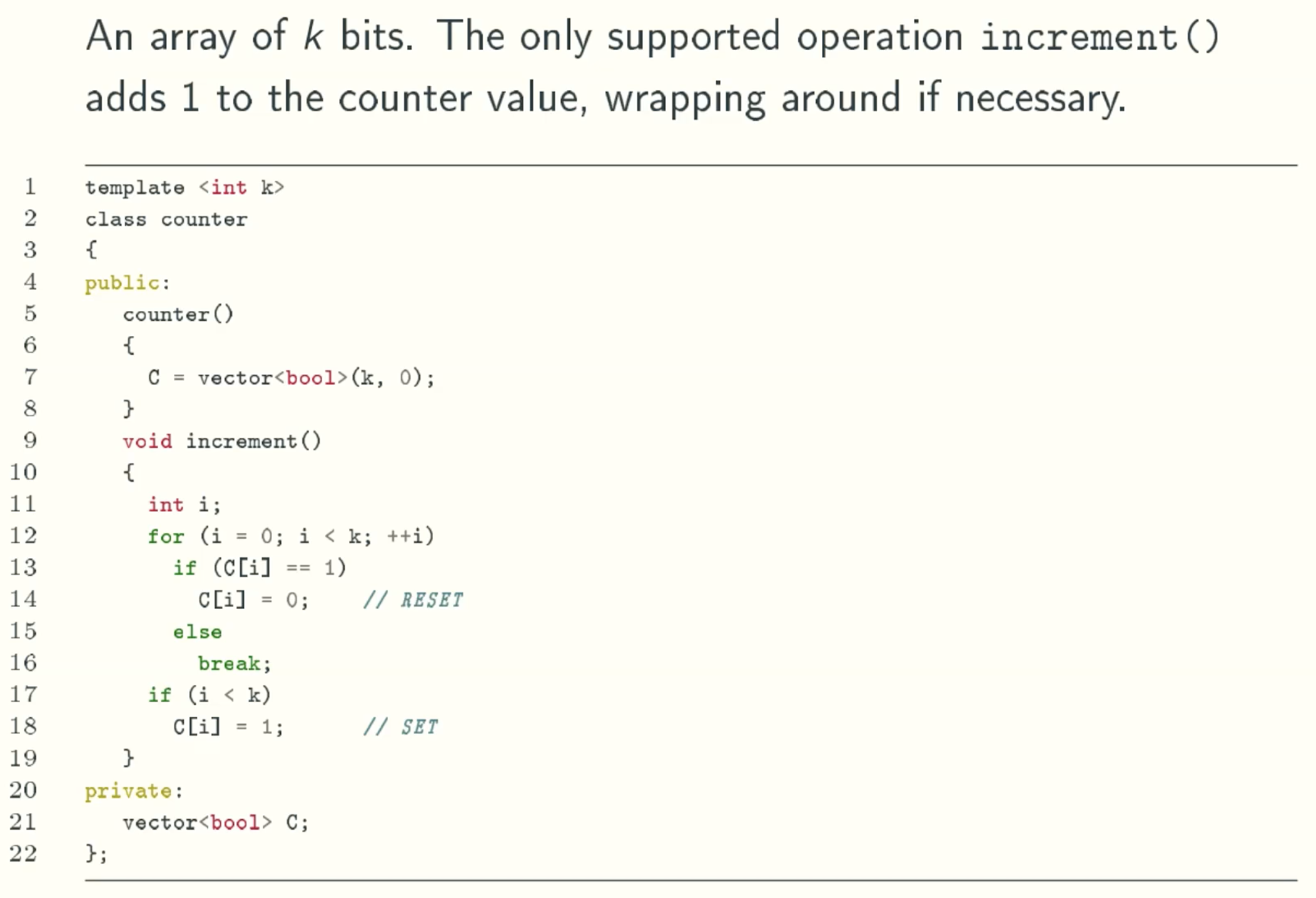
A Toy Example: The K-bit Binary Counter

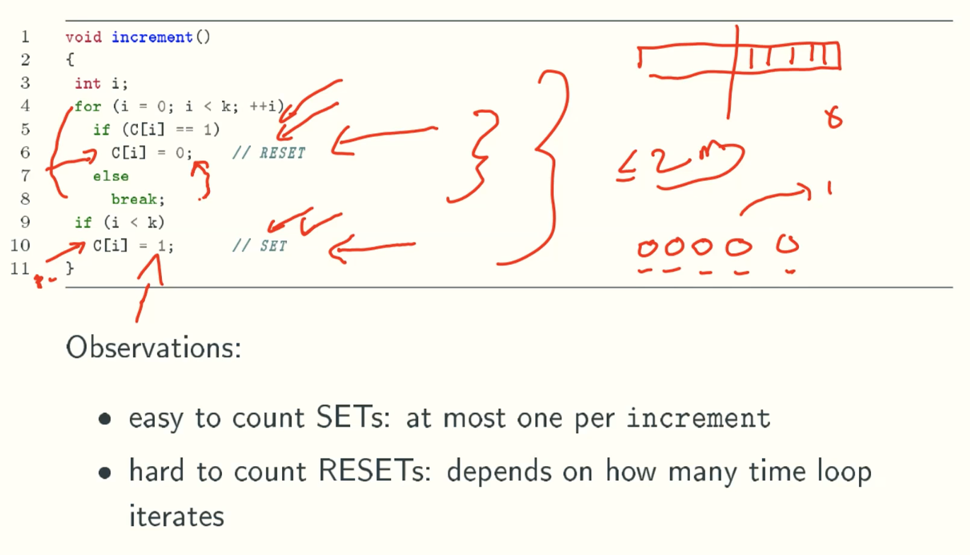
Counter Data Structure

Traditional Analysis

The worst running time of one increment is k bit flips.  
The worst running time of m increments is km bit flips.  
However, from real running in reality, the running time of m increments is 2m bit flips.

How to get the correct result?

Amortized Analysis

Aggregate counting

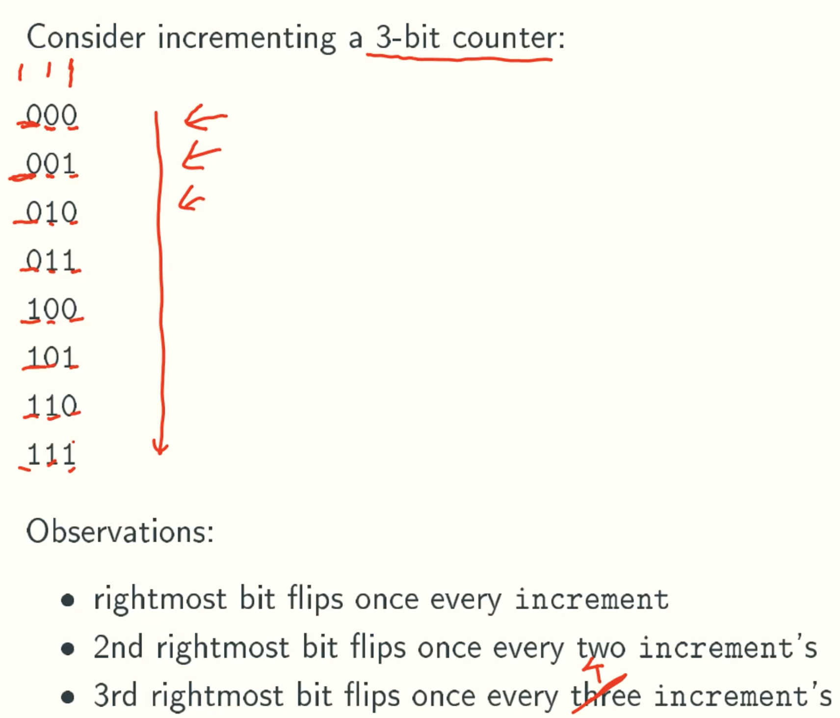
Generalizing: bit i flip once evert 2ⁱ increment’s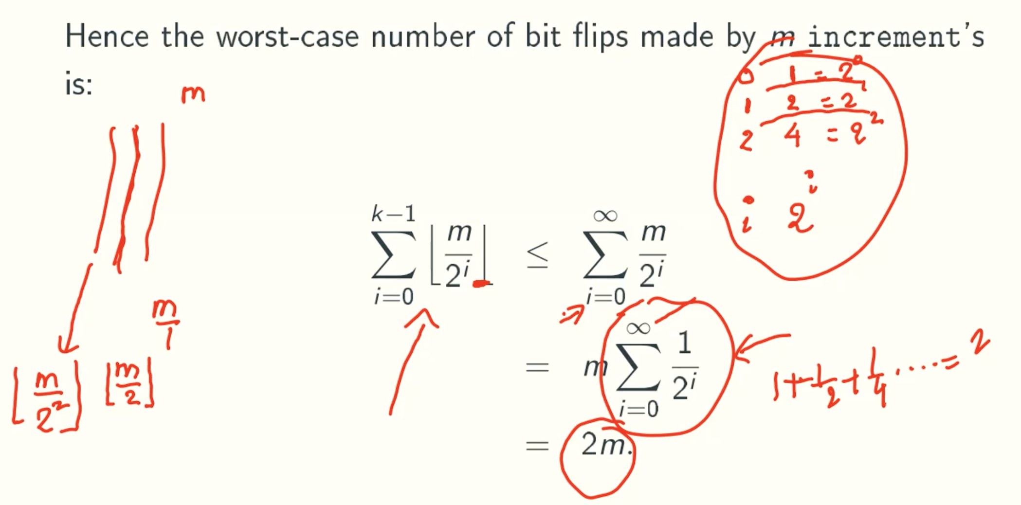

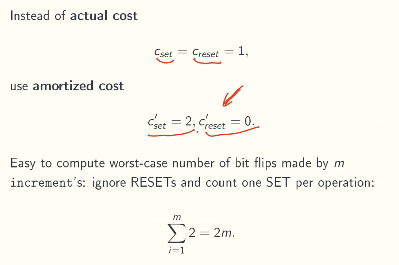
Funny accounting

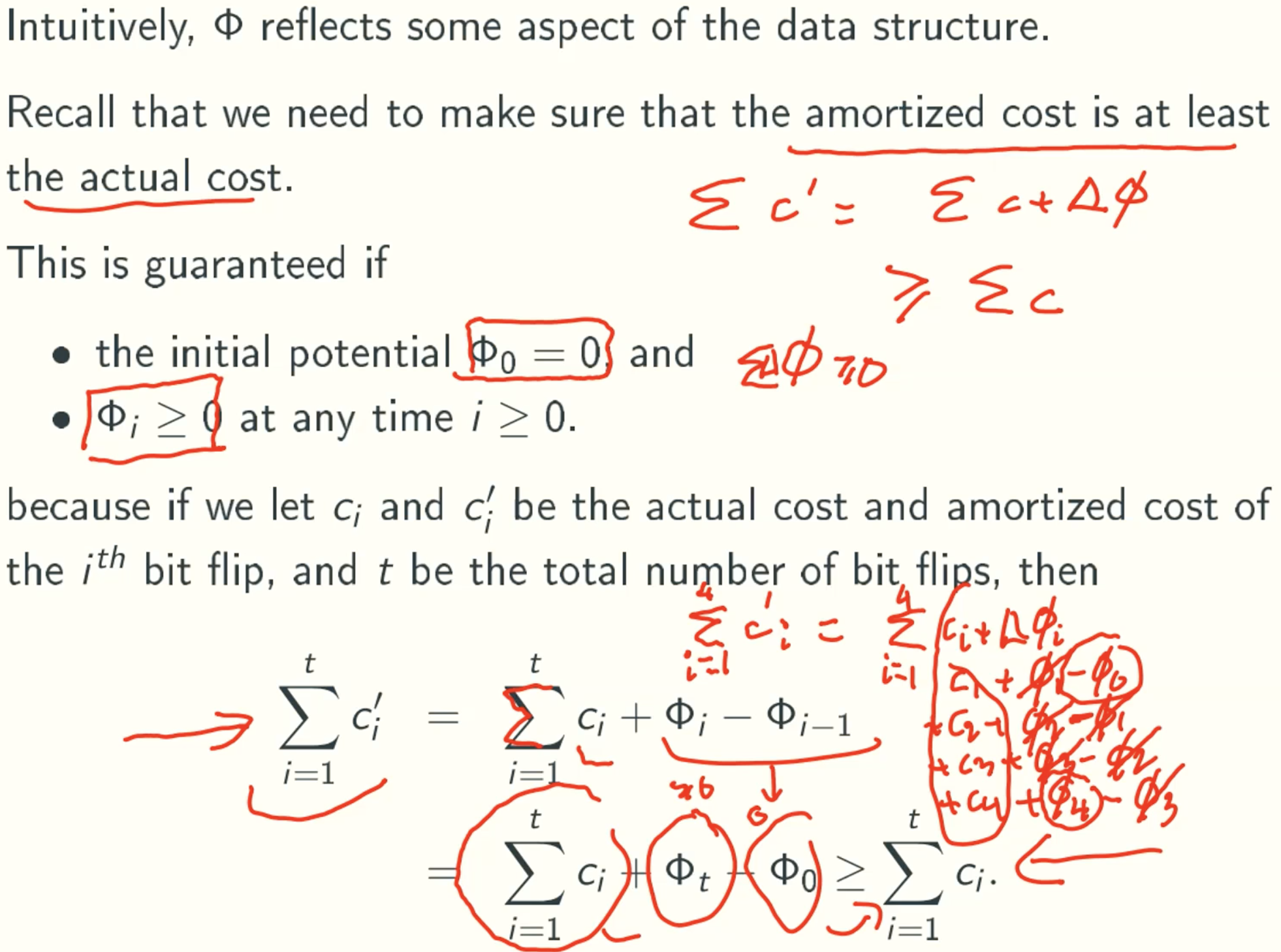
Why amortized cost >= acutal cost
That is because reset operations occurs after set operations.

Potential function

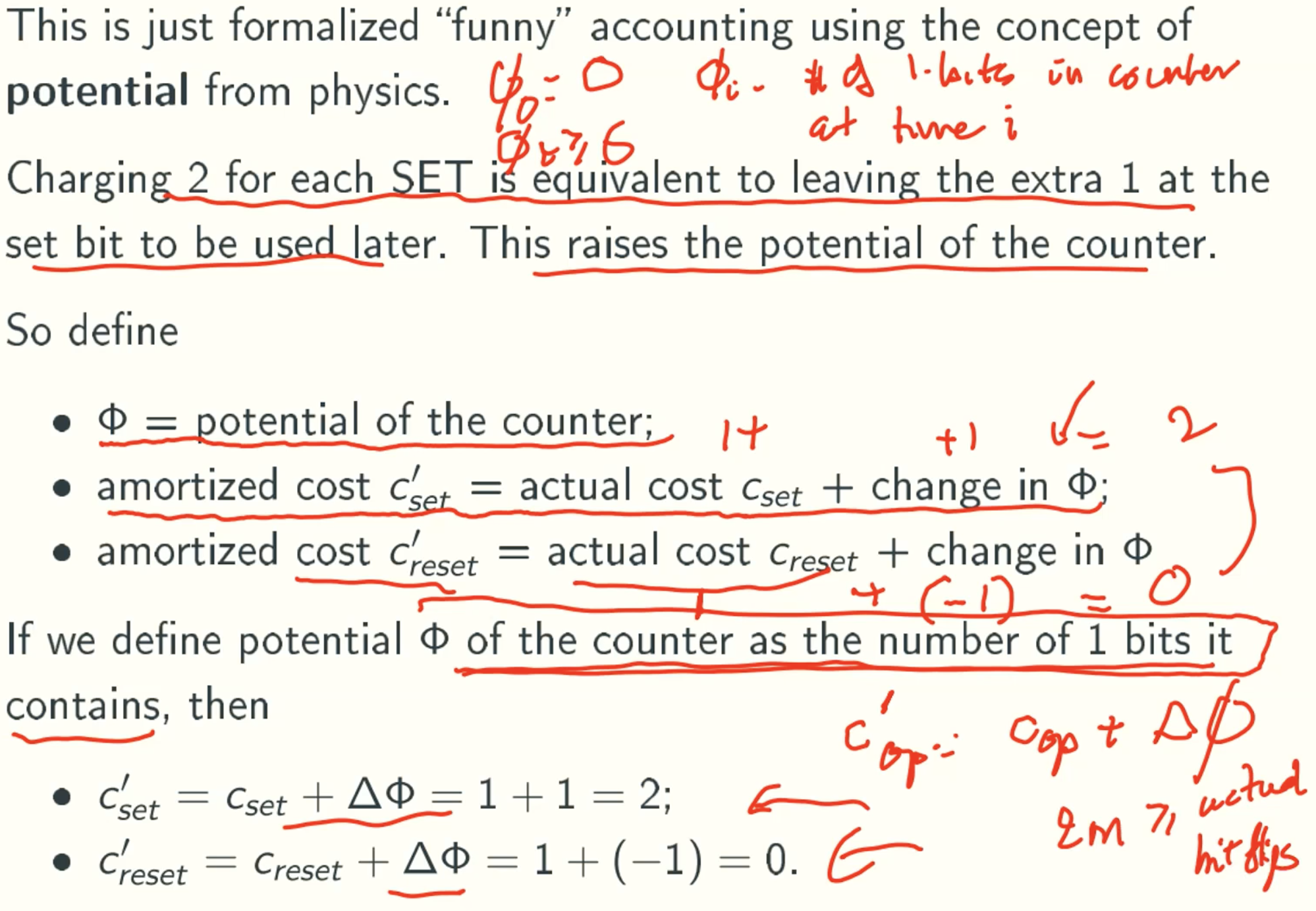
How to pick φ？

Note
C_i = C_set + C_reset = 2 + 0 = 2.

Dynamic Stacks

Data Structure

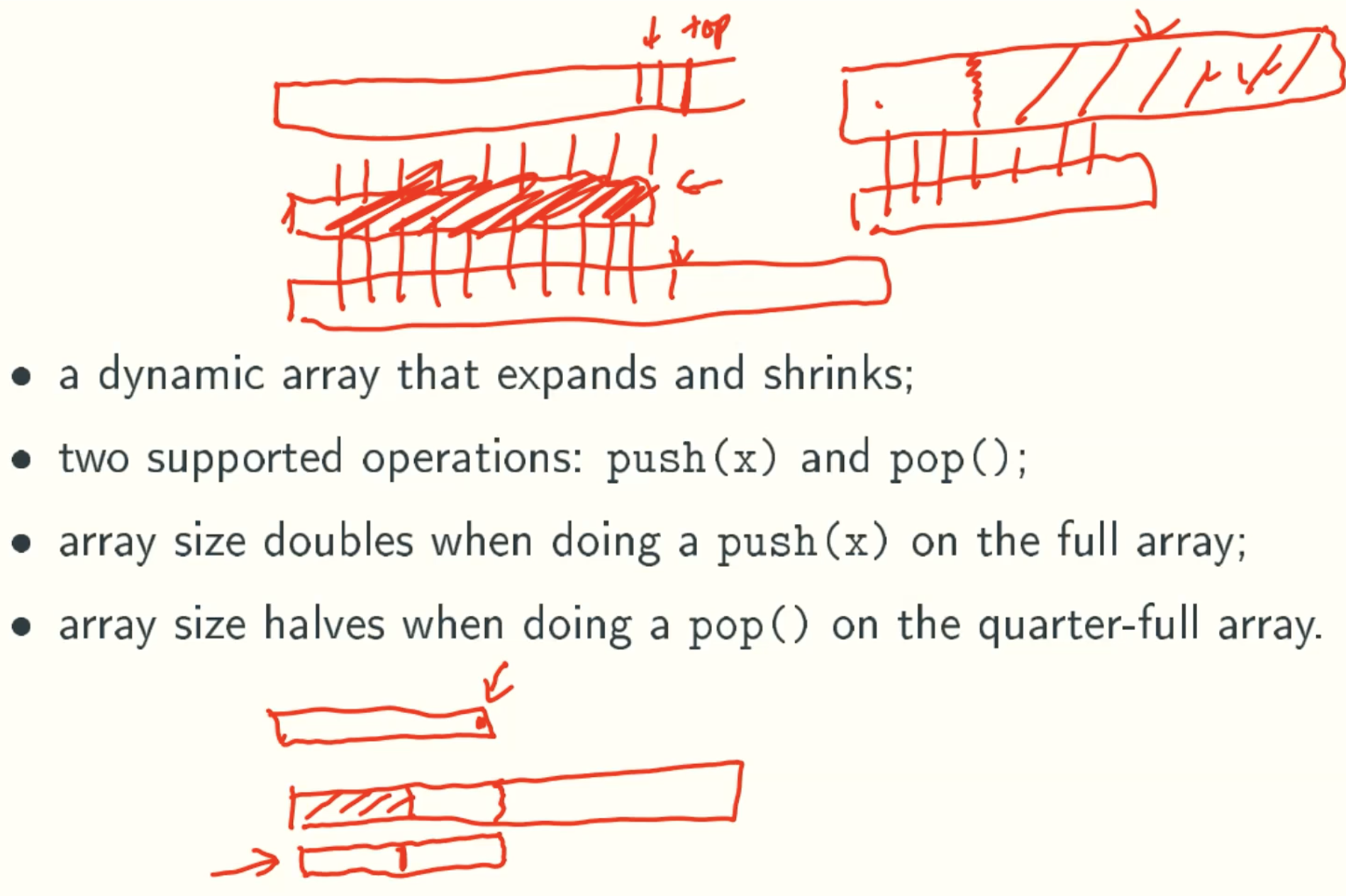
Implementation

Definition

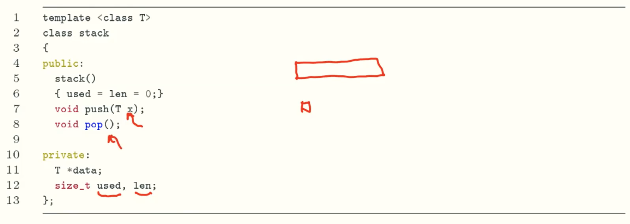
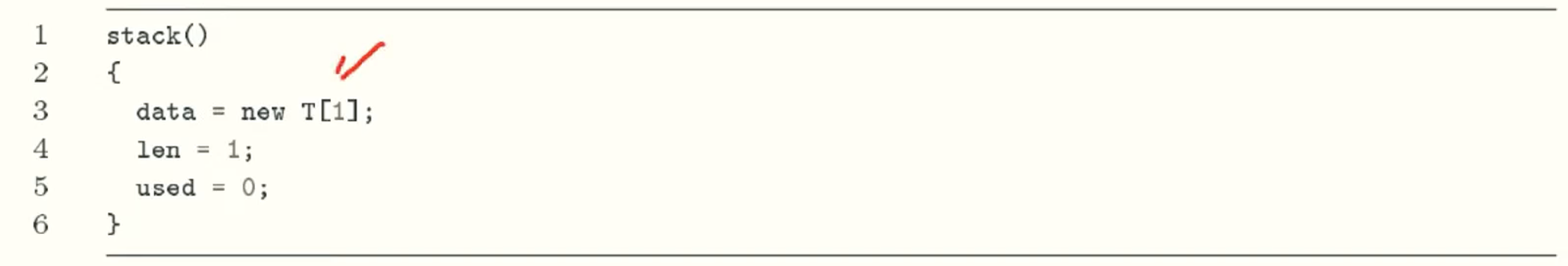
Constructor

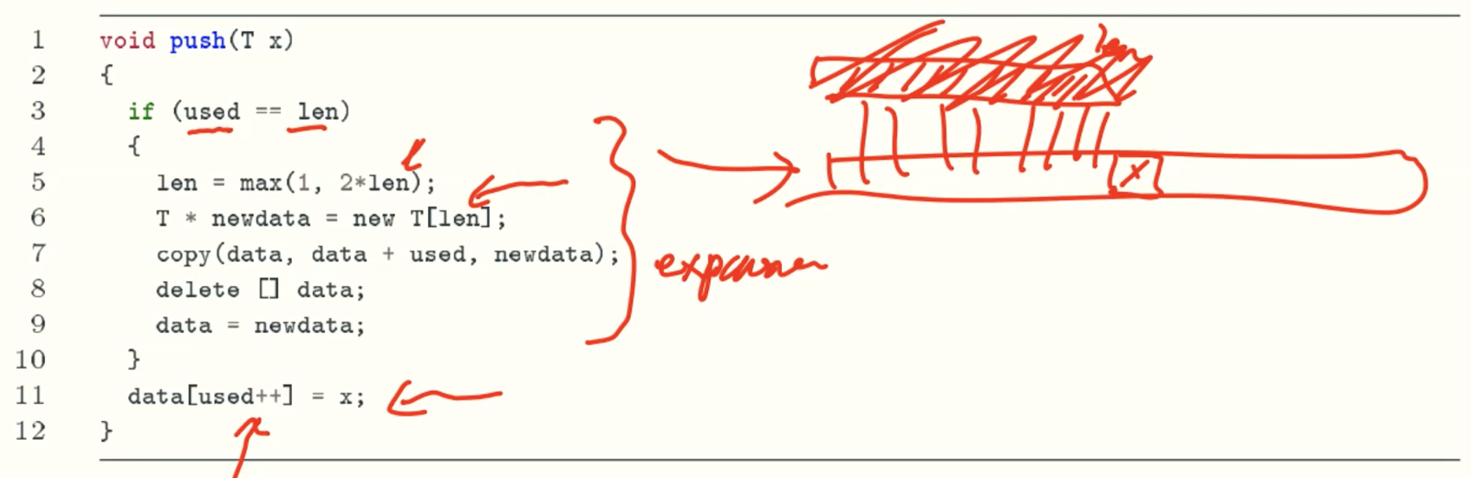
Push

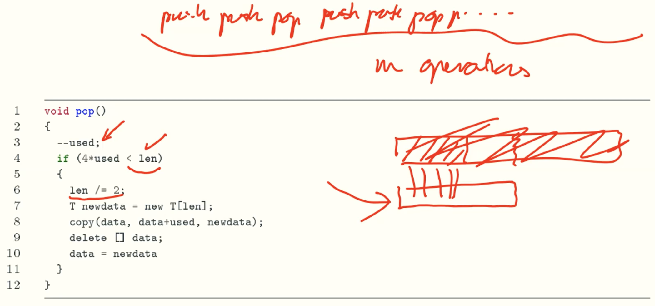
Pop

Traditional Analysis

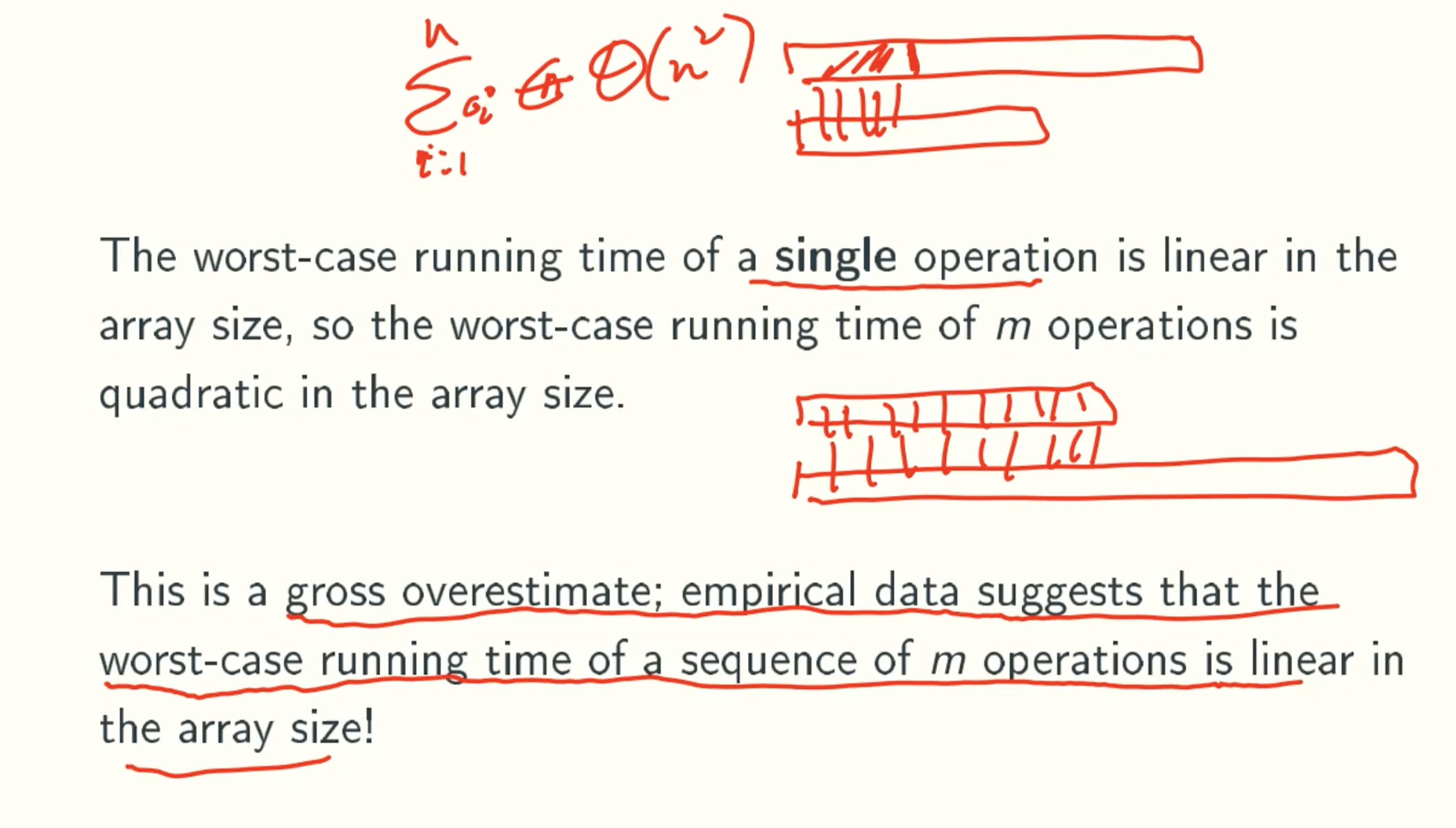
The worst running time of one operation is linear of array size
The worst running time of m operations is ∑(i= 1 to m) i = φ(m²)
However, from real running in reality, the running time of m operations is linear in array size

Amortized Analysis

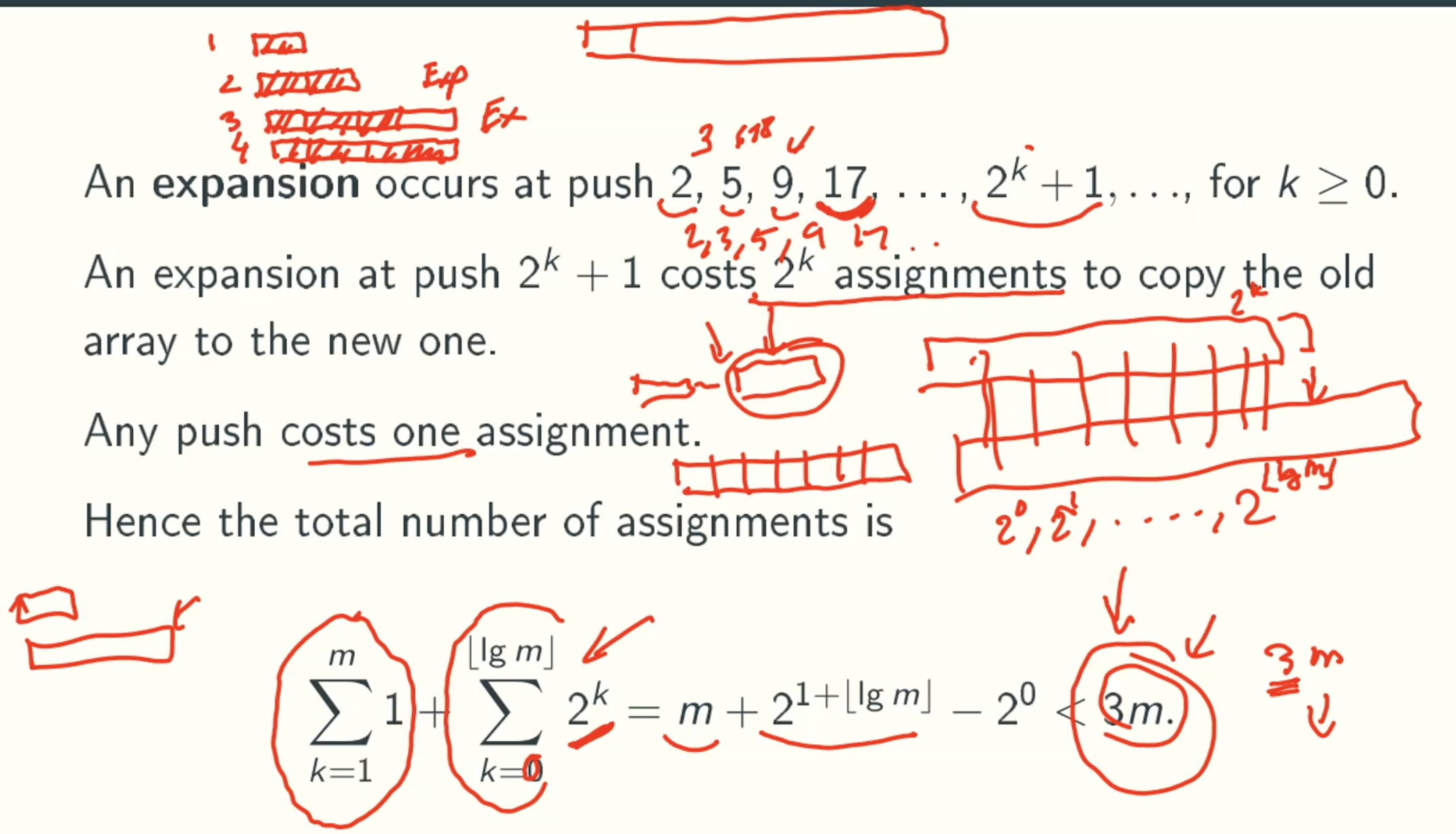
Example: m pushes

Aggregate counting

Q&A

1. Why we use lg(m) rather than lg(m-1) here, Two to the power doesn’t need any new expansion?
   Because we calculate upper bound here. It just use lg(m) for convenience.

2. ∑(k=1 to m)1 + ∑(k=0 to ⌊lg(m)⌋) 2^k = m + 2^{1+⌊lg(m)⌋} - 2⁰ < 3m?

   ∑(k=0 to ⌊lg(m)⌋) 2^k = 1*(1-2^{lg(m) + 1})/(1-2) = 2^{lg(m) + 1} - 1.

   2^{lg(m) + 1} - 1 = 2*2^lg(m) - 1= 2m - 1

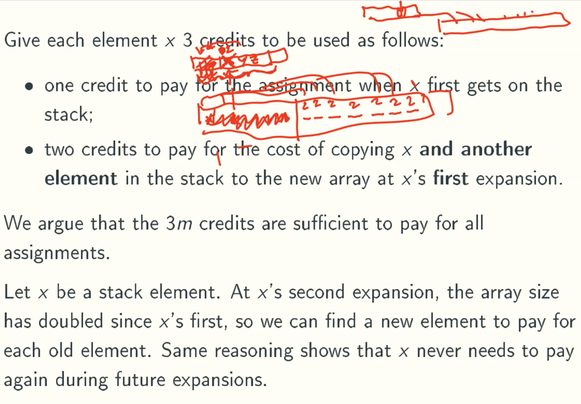
Funny accounting

Potential function

φ here mean the change in the credits we have in i_th push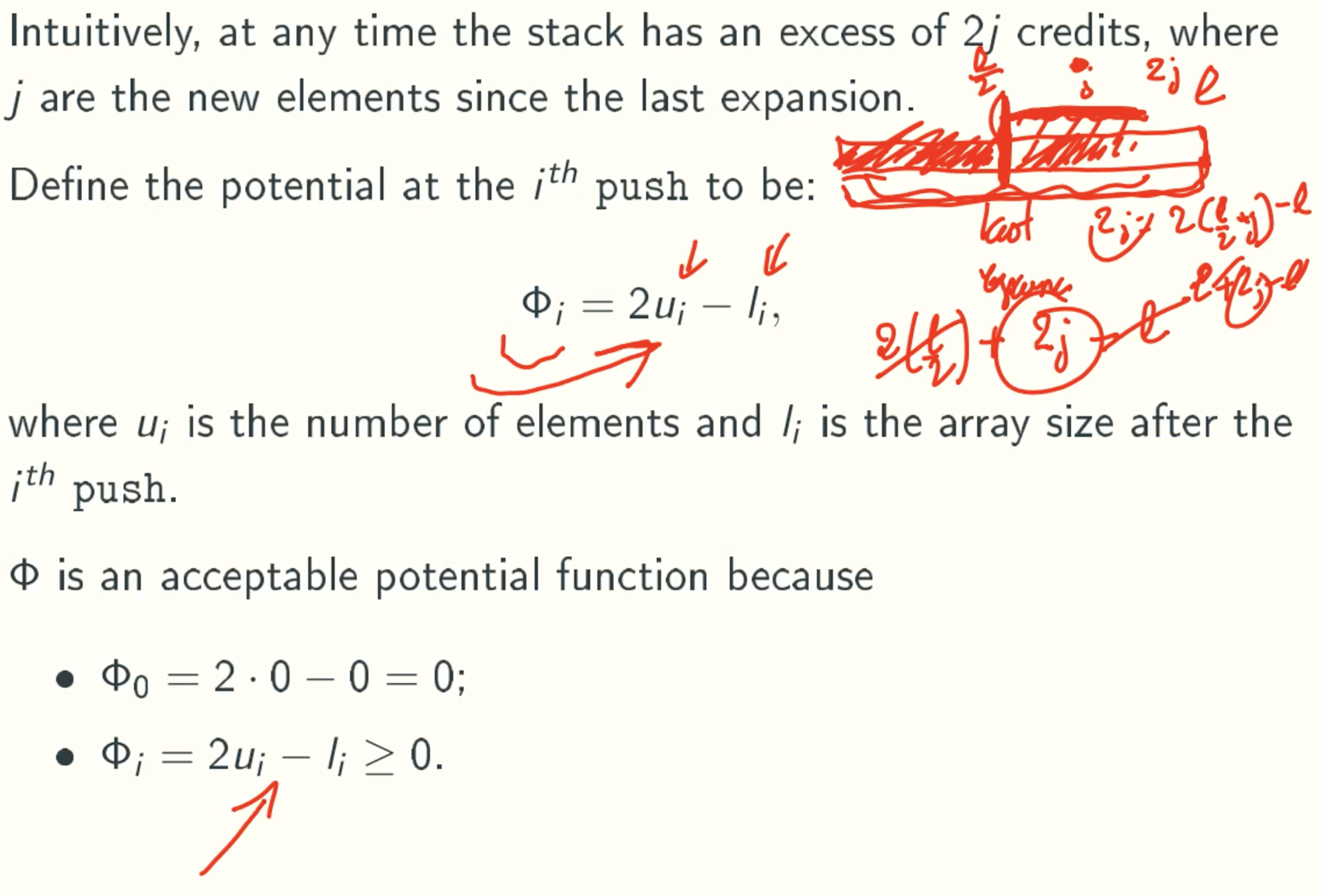

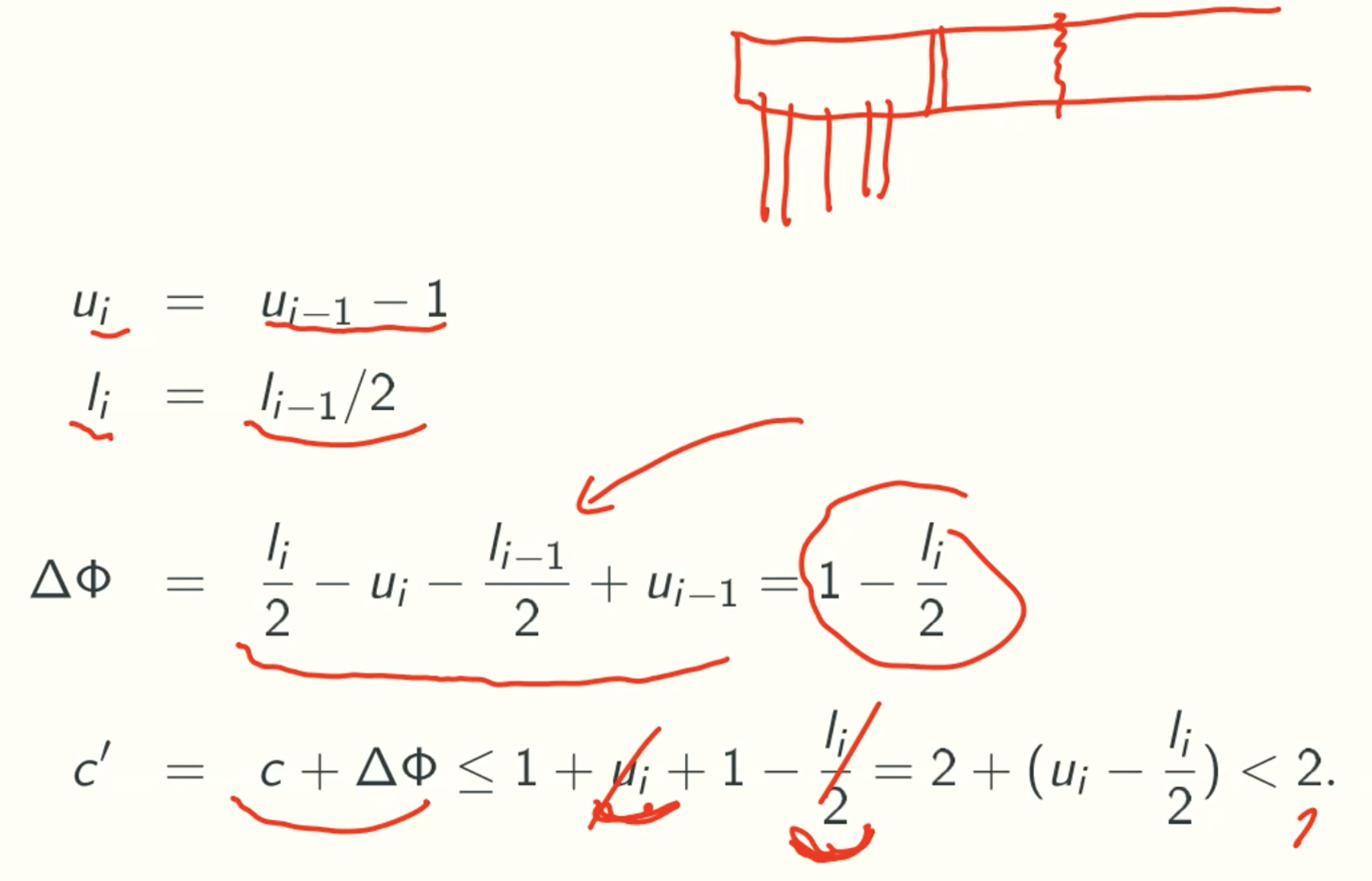
Example: general case of m push/pop operations

Potential function

φ here mean the change in the credits we have in i_th push/pop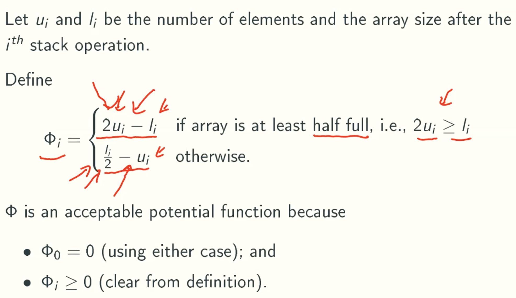

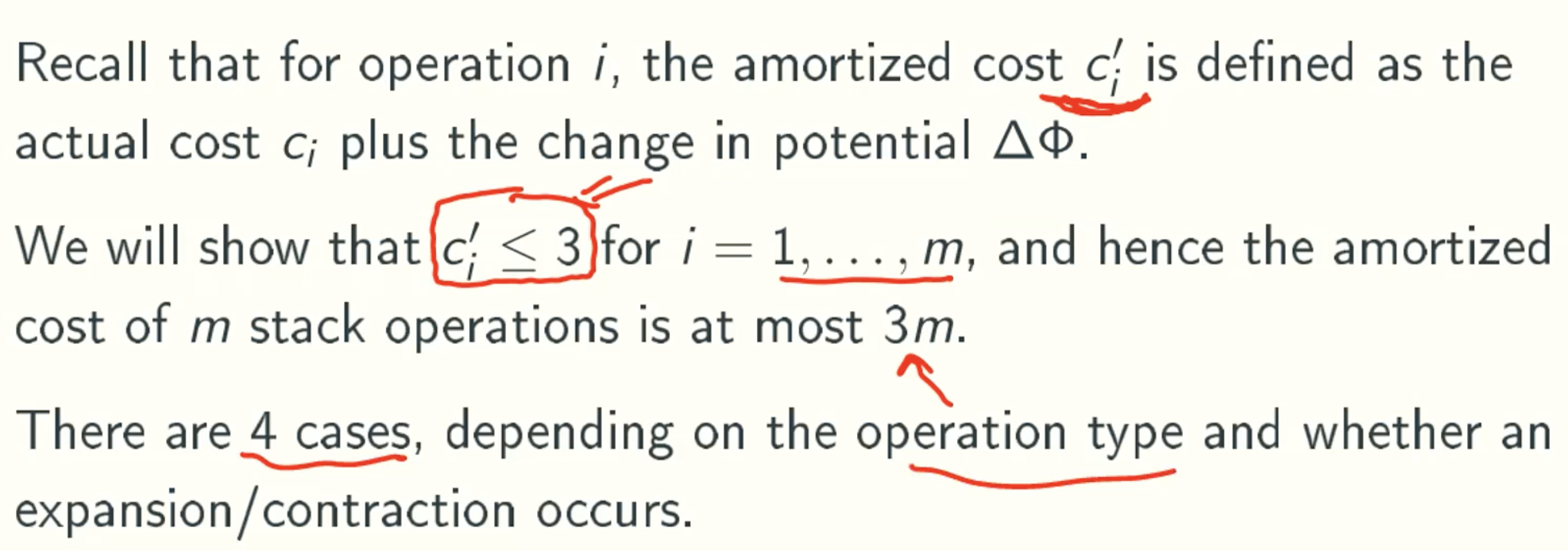
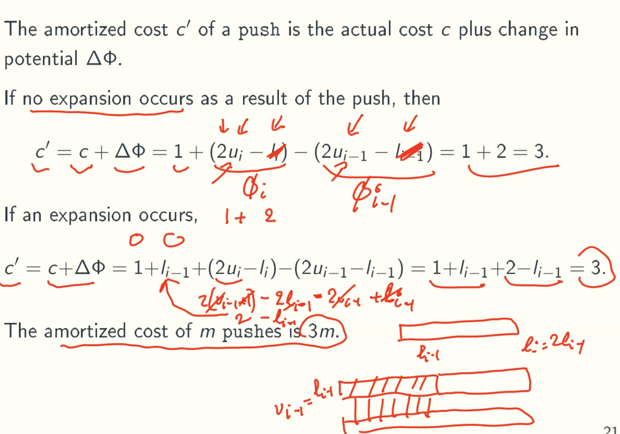
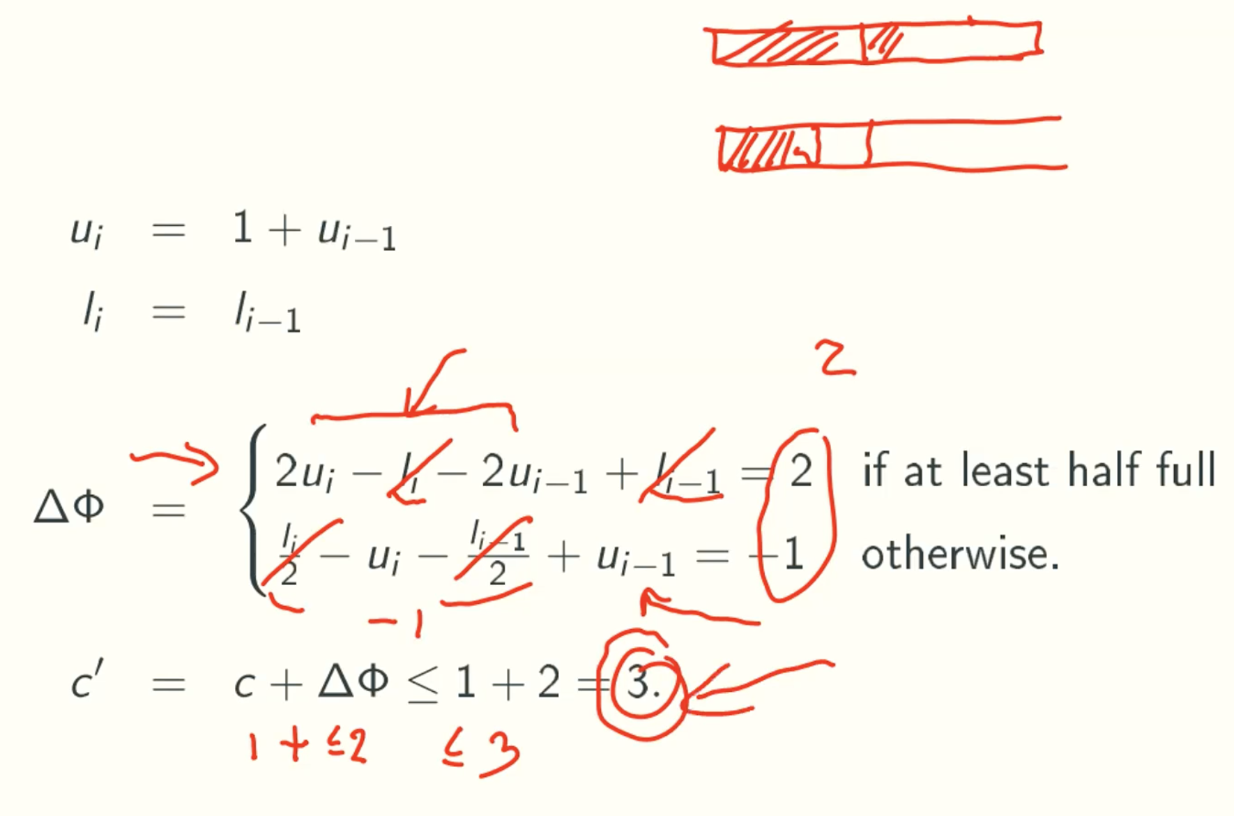
1. push without expansion
   
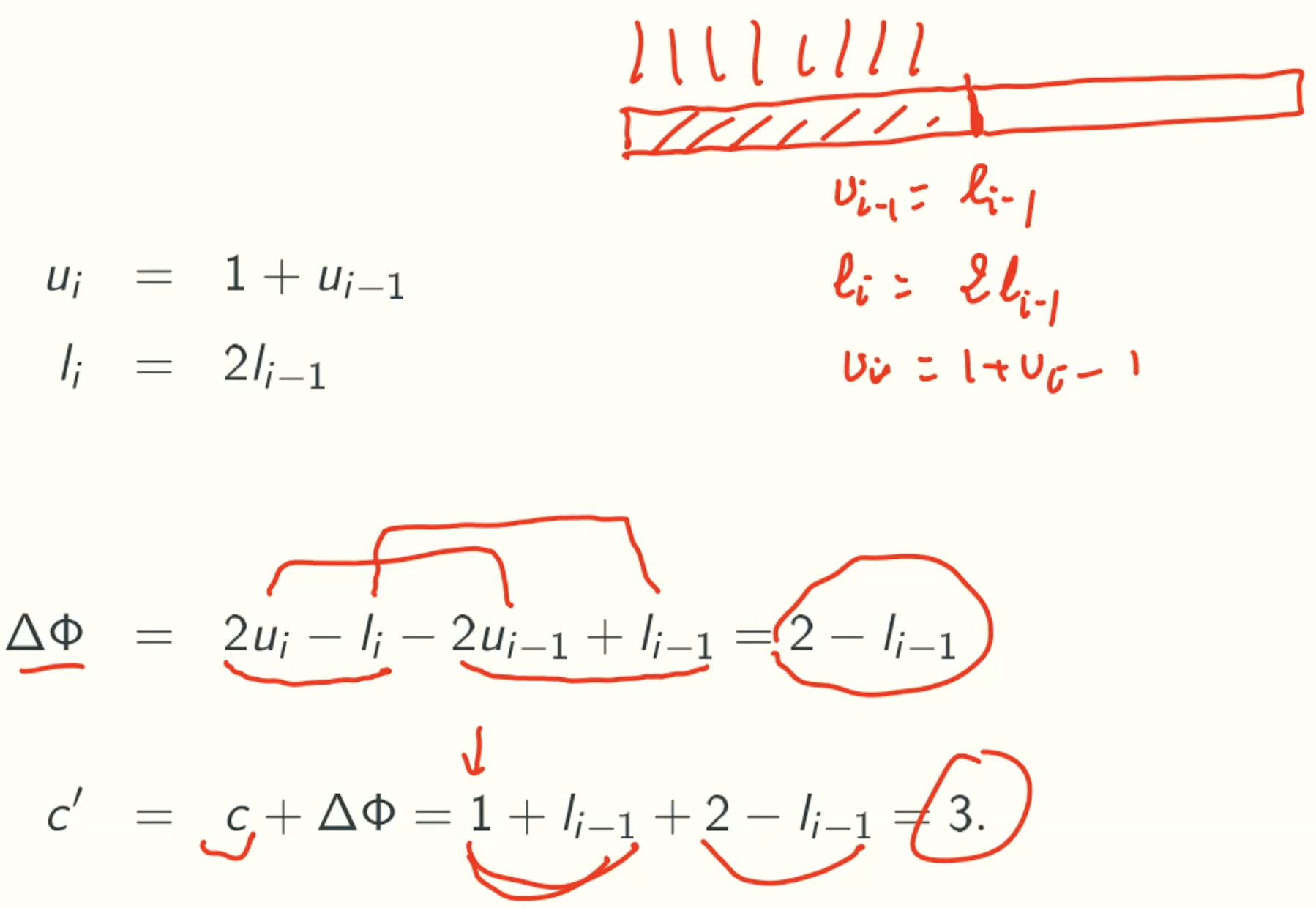
2. push with expansion
   
3. pop without contraction
   
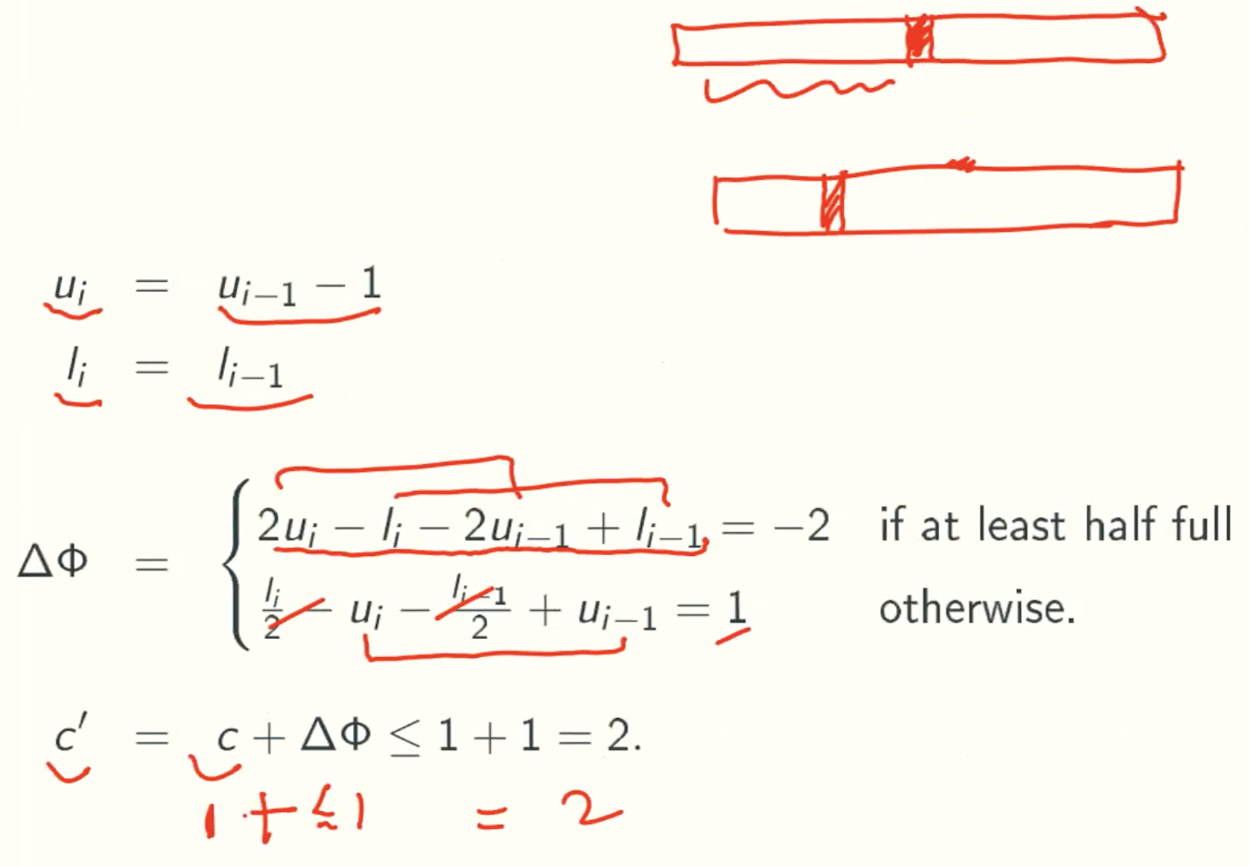
4. pop with contraction
   

UNIVERSAL HASHING

Dictionary Problem

Problem Definition

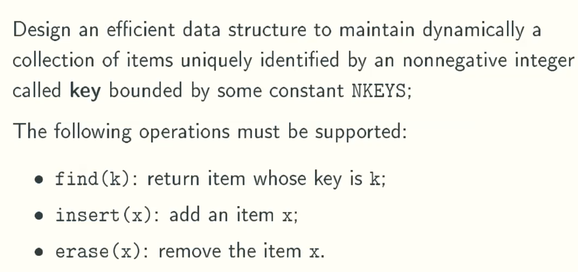
Royal Solution: Use An Array Of Size NKEYS

Implementation

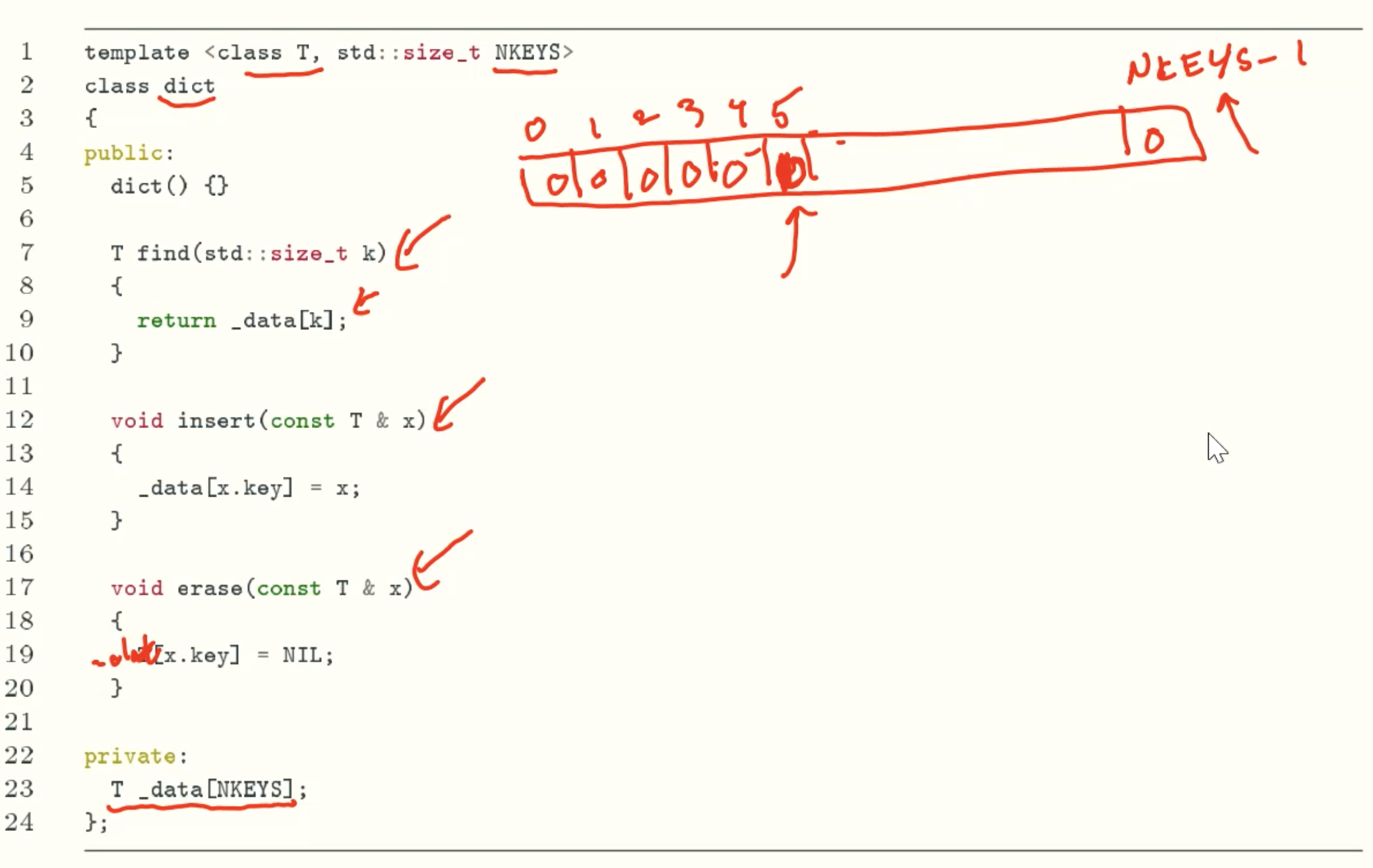
Analysis

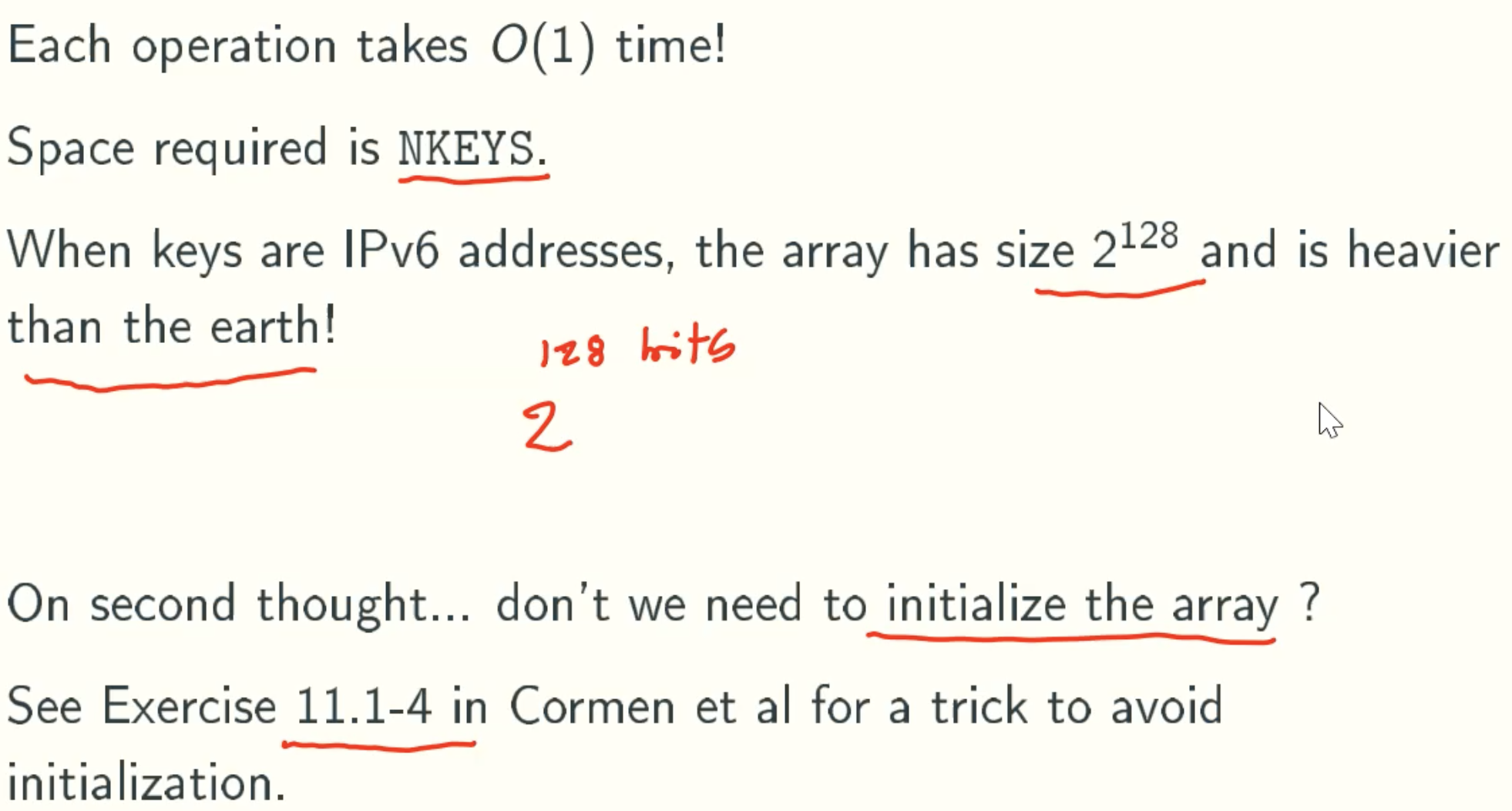
11.1-4
We wish to implement a dictionary by using direct addressing on a huge array. At the start, the array entries may contain garbage, and initializing the entire array is impractical because of its size. Describe a scheme for implementing a direct- address dictionary on a huge array. Each stored object should use O(1) space; the operations SEARCH, INSERT, and DELETE should take O(1) time each; and initializing the data structure should take O(1) time. (Hint: Use an additional array, treated somewhat like a stack whose size is the number of keys actually stored in the dictionary, to help determine whether a given entry in the huge array is valid or not.)

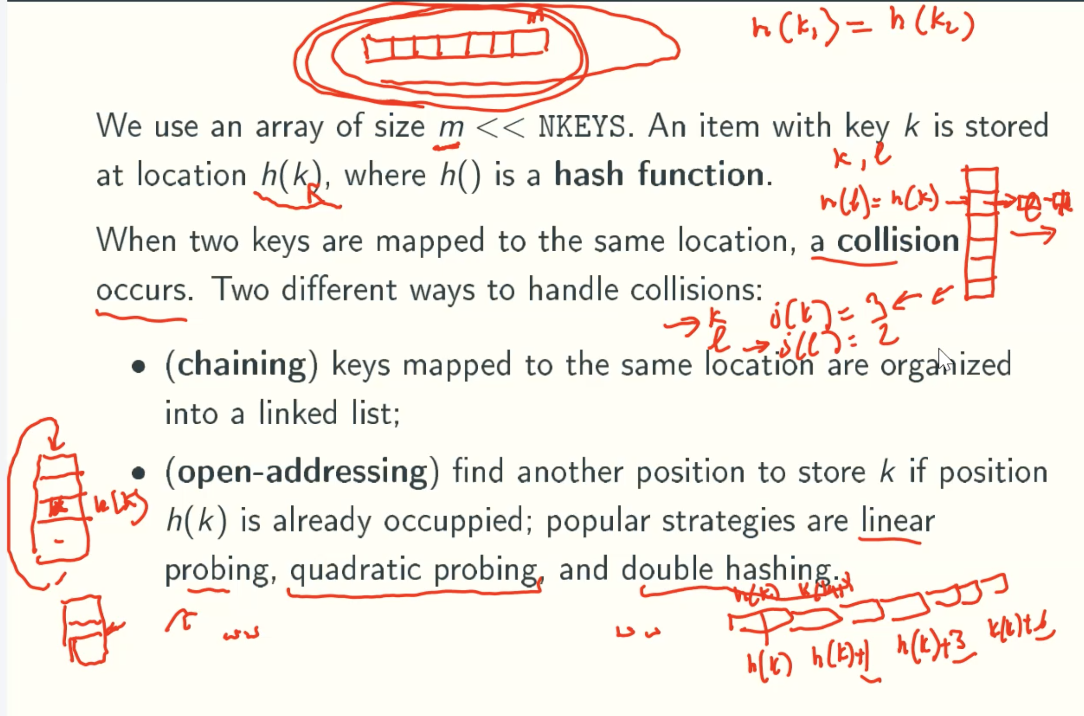
Compromise Solution: Hash Table

Implementation

Quadratic_probing
Double Hashing
Double hashing is a collision resolving technique in Open Addressed Hash tables. Double hashing uses the idea of applying a second hash function to key when a collision occurs

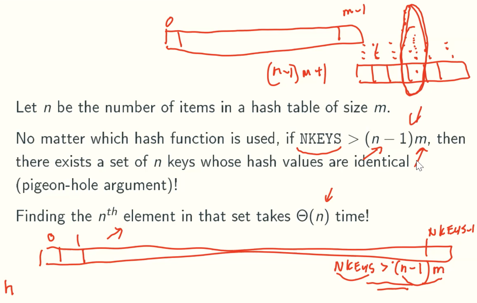
Worst-case Analysis

Average-Case Analysis: chain hashing

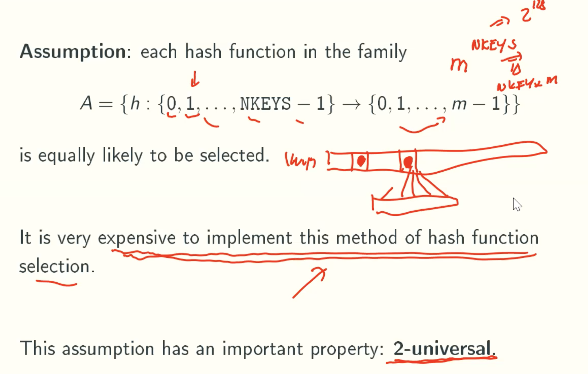
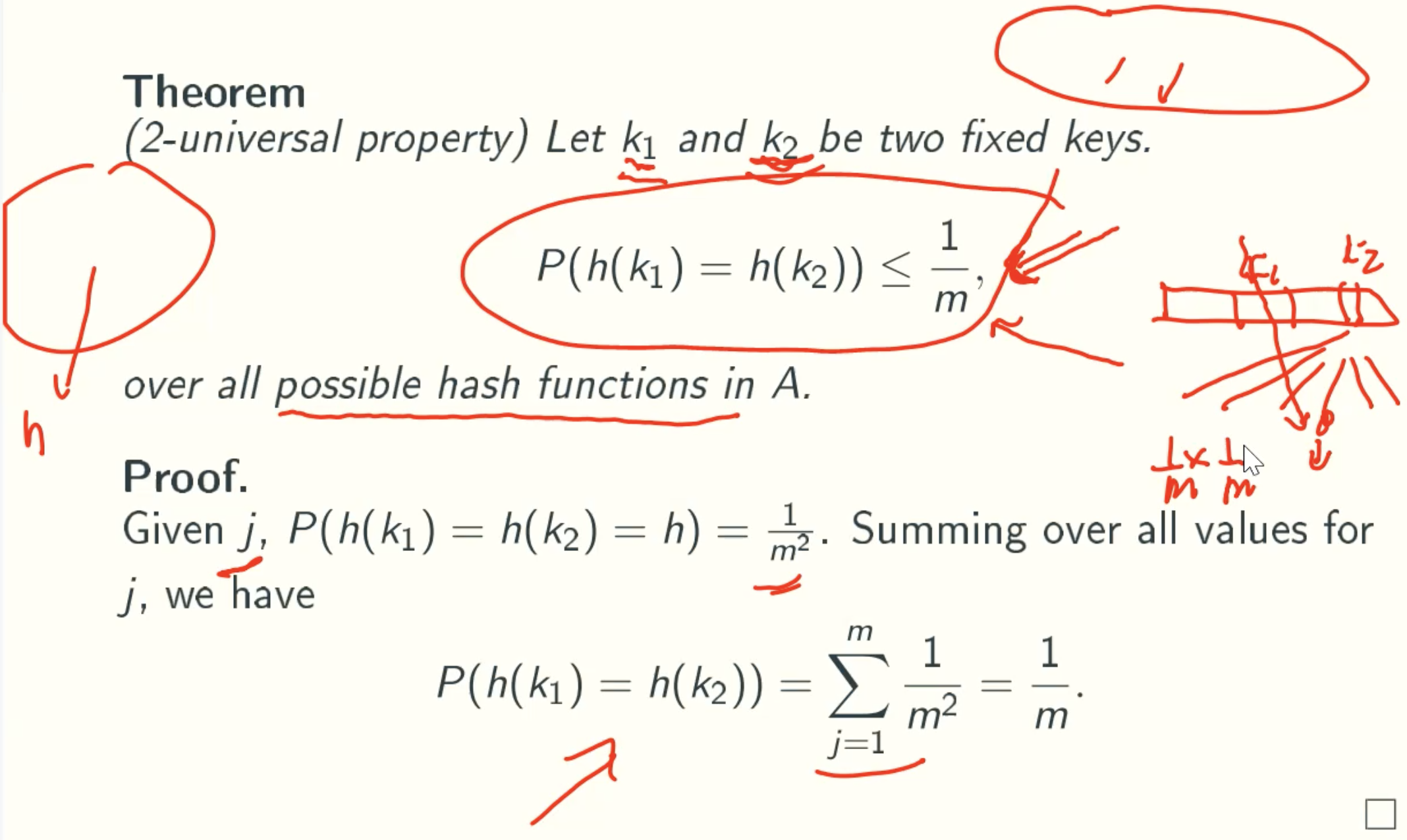
2-Universal Property

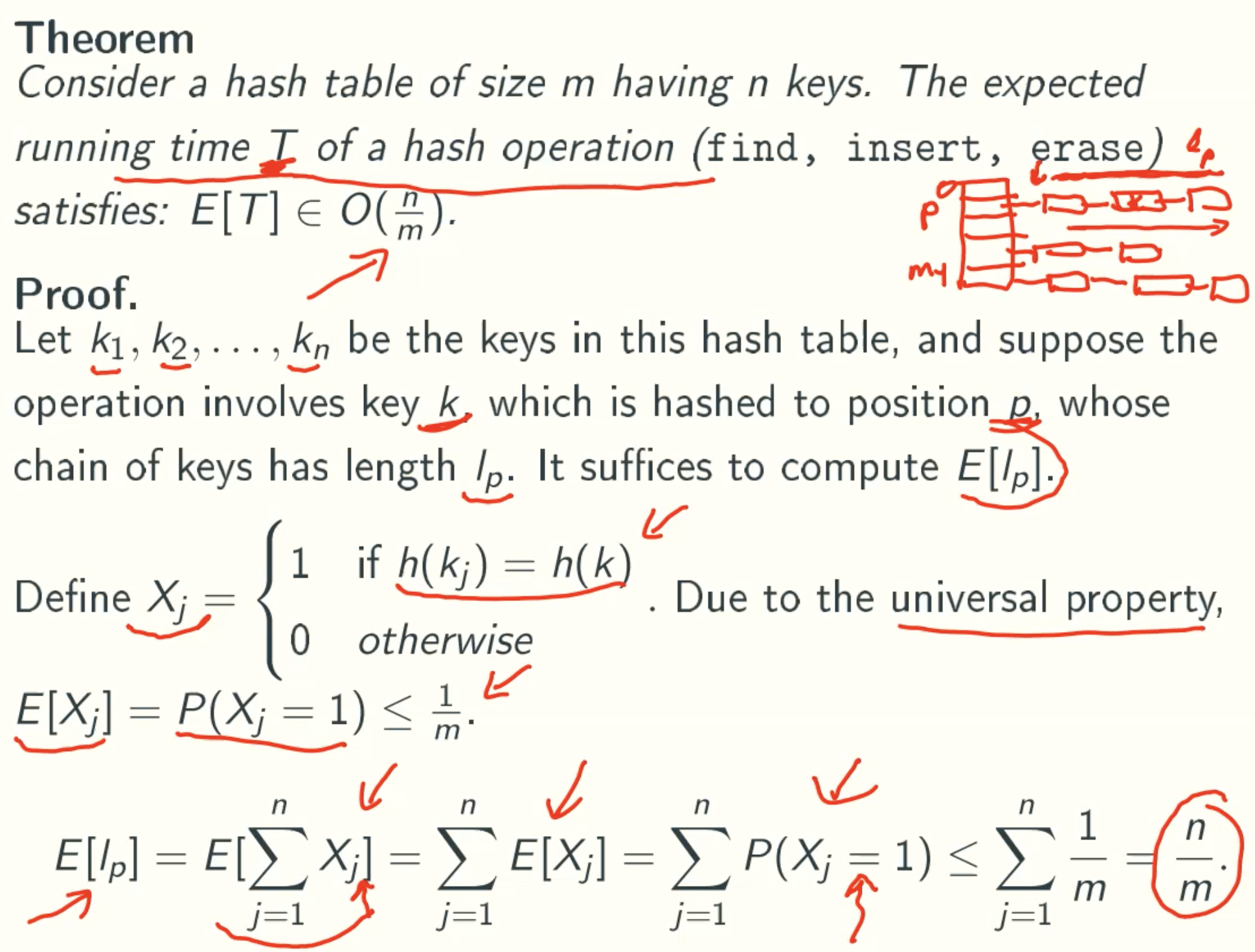
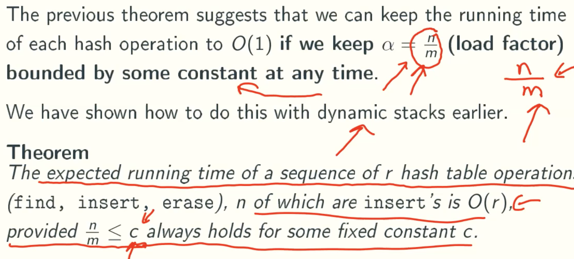
Expect Running Time

Expect Running Time Of A SEQUENCE Of Hash Operation

A Universal Hash Function Family

Universal Property

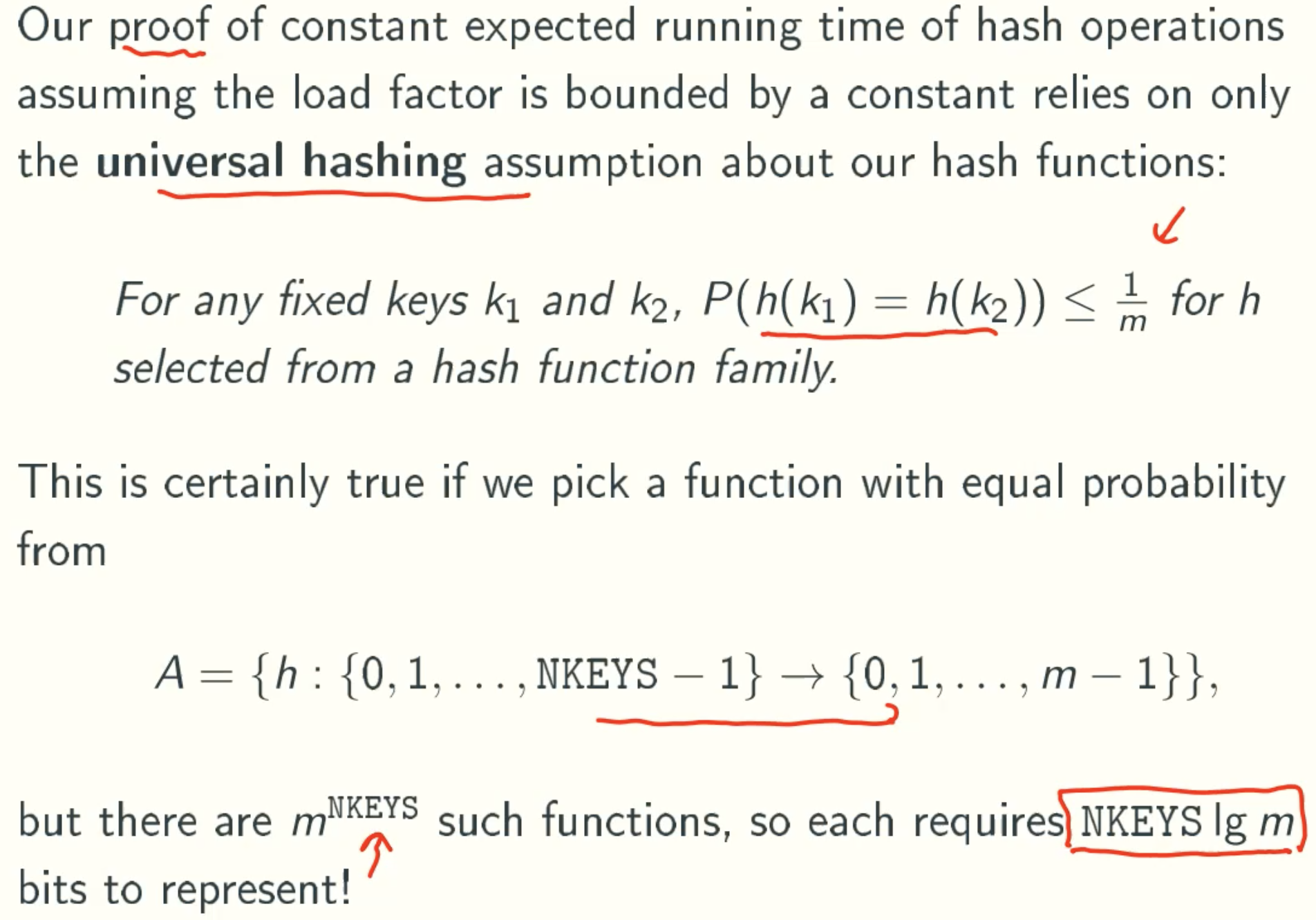
A Much Smaller Family With Universal Hashing Property

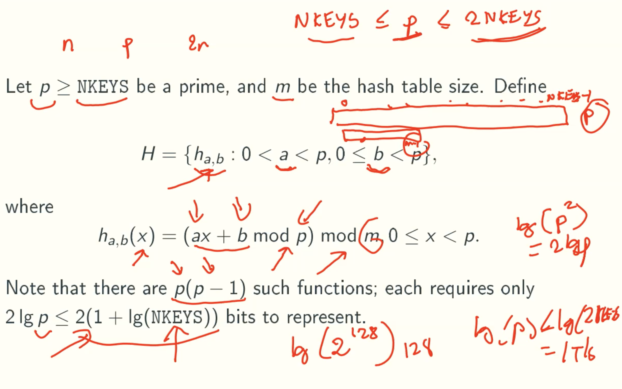
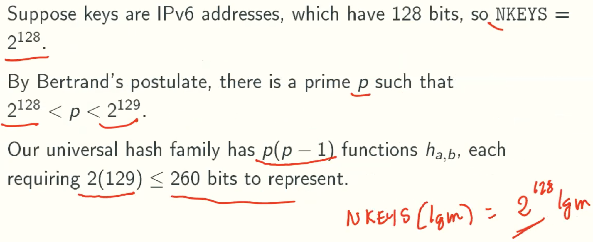
Example

Proof Of Universal Hashing Property

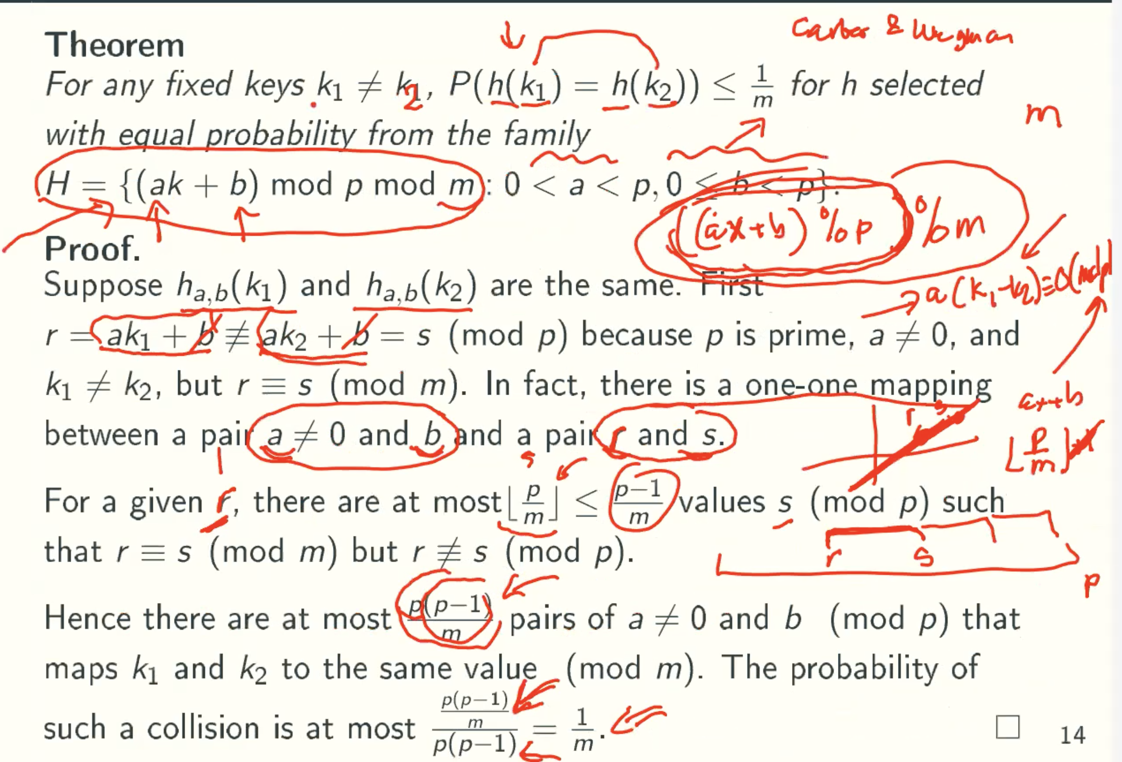
1. ak₁+b ≠ ak₂+b
   Same a,b. Different k, the equation is impossible same.
2. ak₁+b ≠ ak₂+b mod P
   If ak₁+b = ak₂+b mod P
   Then a(k₁-k₂) = 0 mod P
   Since P is Prime, so a is 0 or k₁=k₂. However, a is bigger than 0, and k1 ≠ k2, So it is impossible that ak₁+b = ak₂+b mod P.
3. ak₁+b = (ak₂+b mod P)mod m
   Assume ak₁+b = r, ak₂+b mod P = s.
   If r = s mod m, the difference between r and s is an integer multiple m.
   So there are p/m pairs. And since P is prime, p/m ≤ (p-1)/m. And r can be any numbr for 0 to P. So the total same pairs is p(p-1)/m.
4. The collision probability 1/m.
   k₁ and k₂ has total p(p-1) pairs, so the collision probablity of each pair is p(p-1)/m/(p(p-1)) = 1/m.

Perfect Hashing

Perfect Definition

Given n keys, a hashing function is perfect if it maps each of the key to a unique position.

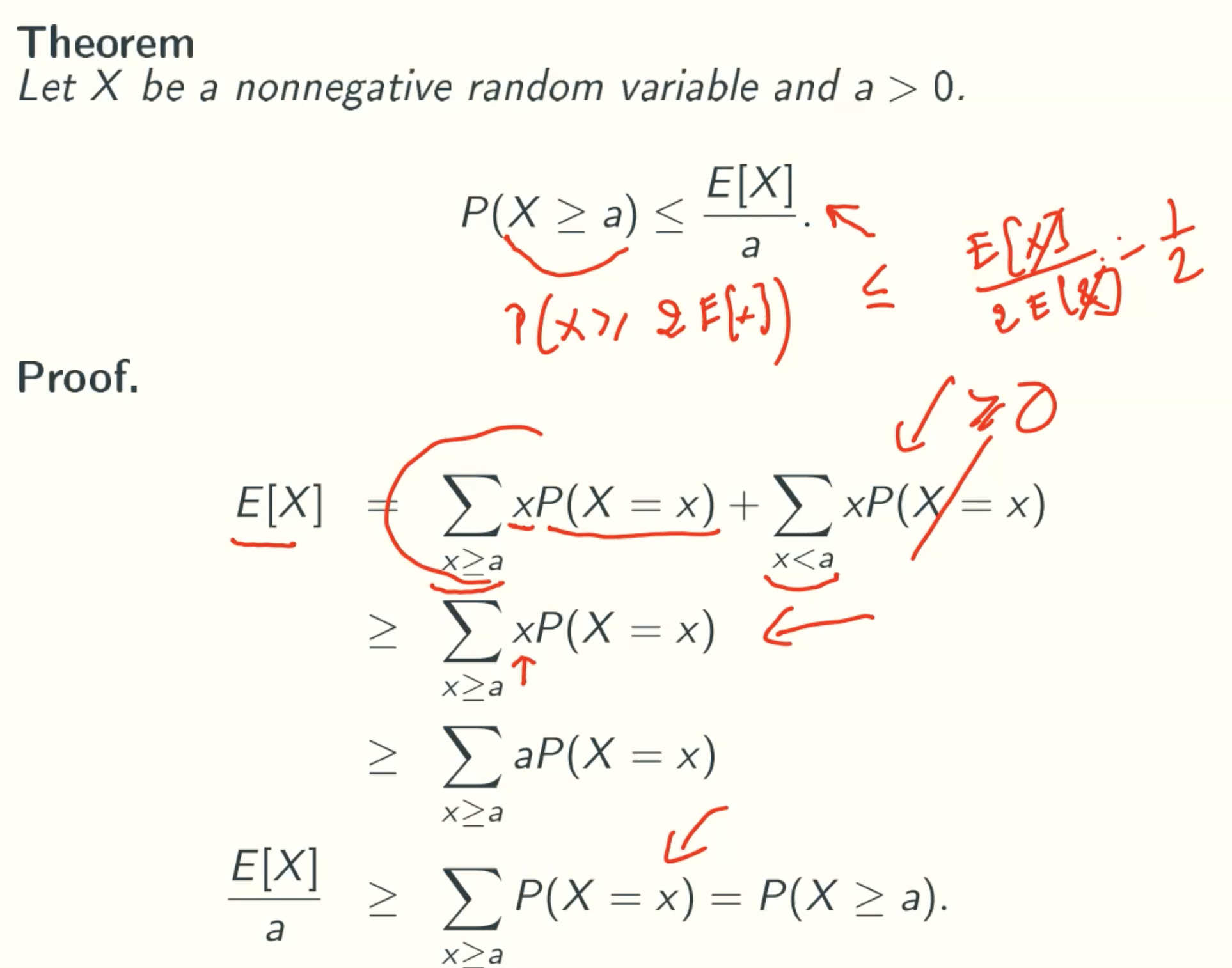
Markov’s inequality

Perfect Hashing using quadratic space

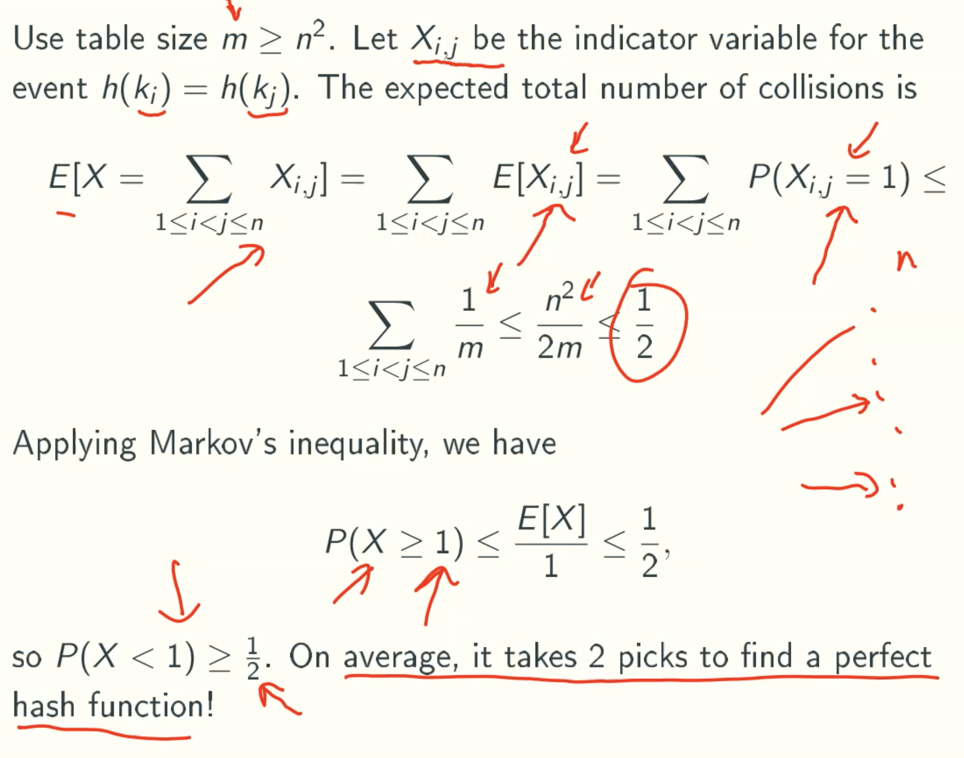
Why ∑ 1/m ≤ n²/m?
loop through all pairs (i,j) = n + (n-1) + (n-2) + … + 1 = (n+1)*n/2

Perfect Hashing using linear space

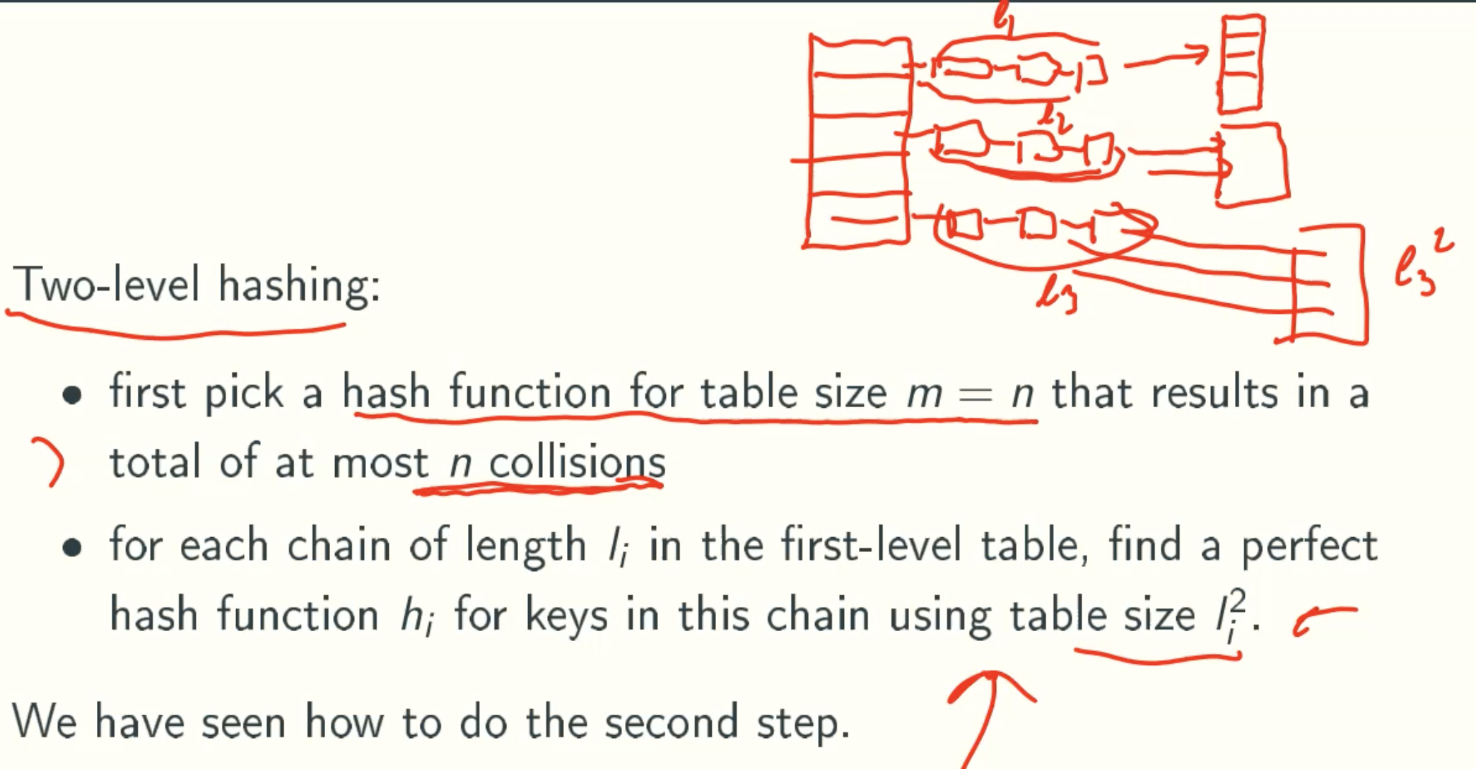
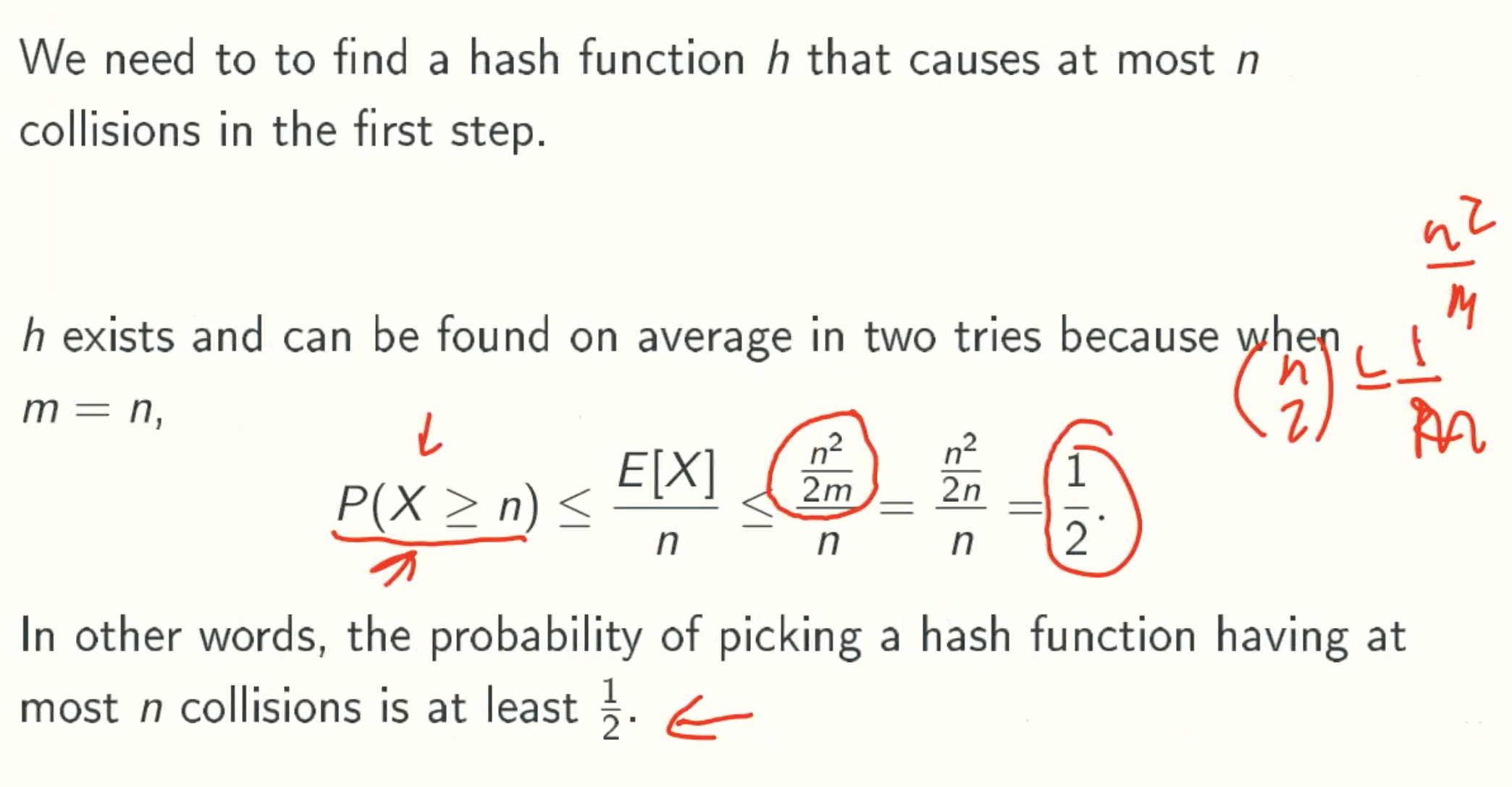
First Step

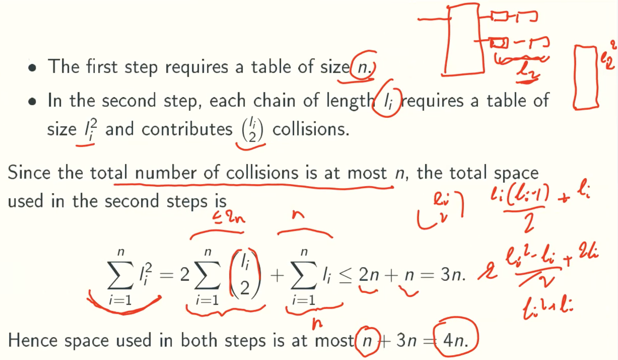
Space Analysis

Binary Search Tree

Extended Dictionary Problam

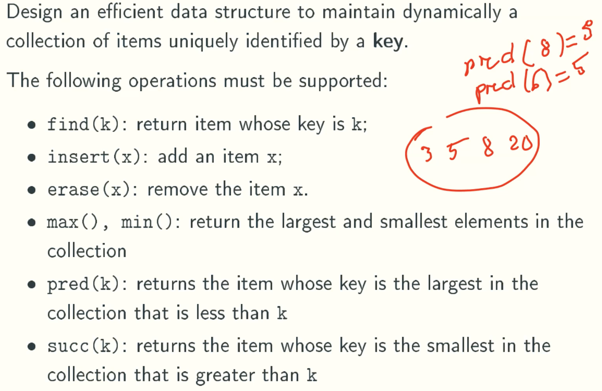
Classical Solution: Binary Search Tree

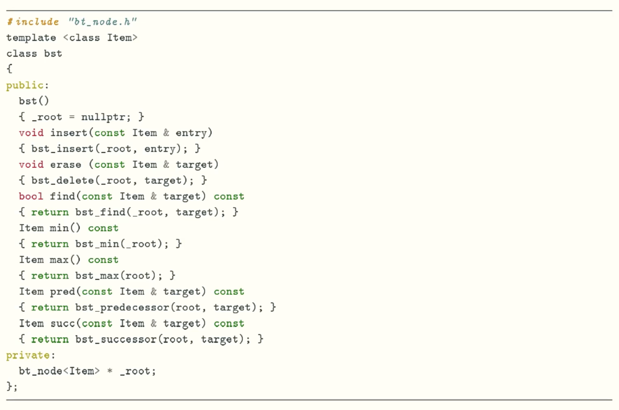
Implementation

Class Definition

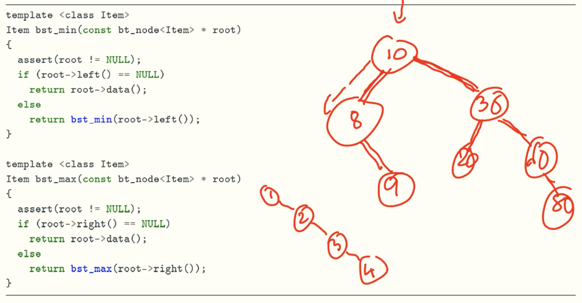
min & max function

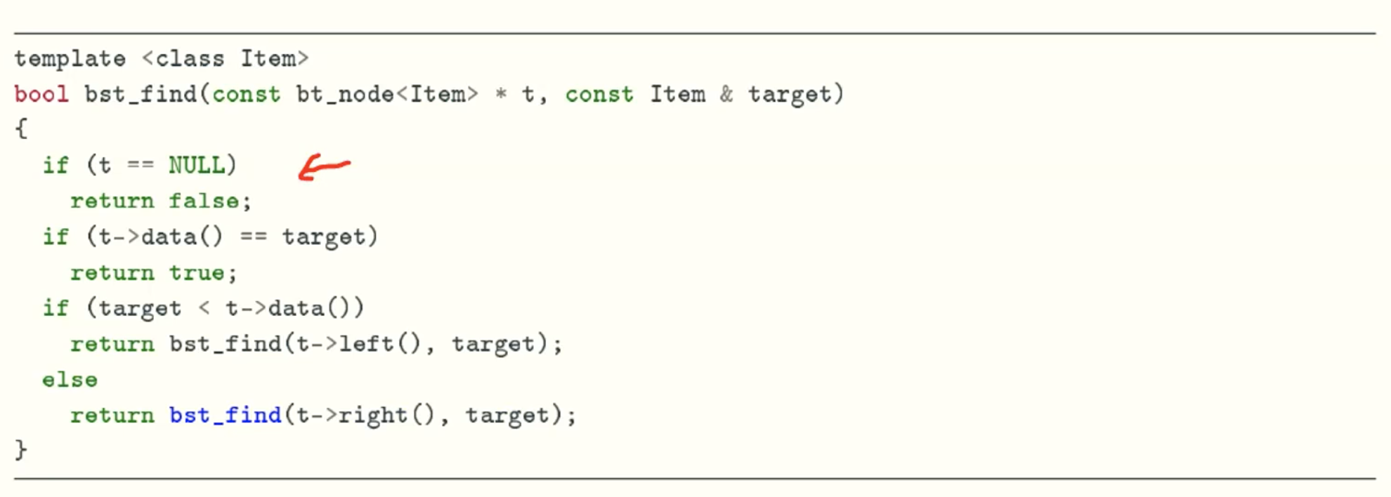
find function

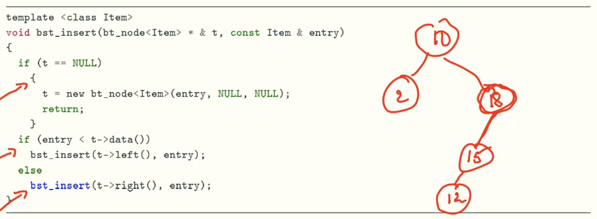
insert function

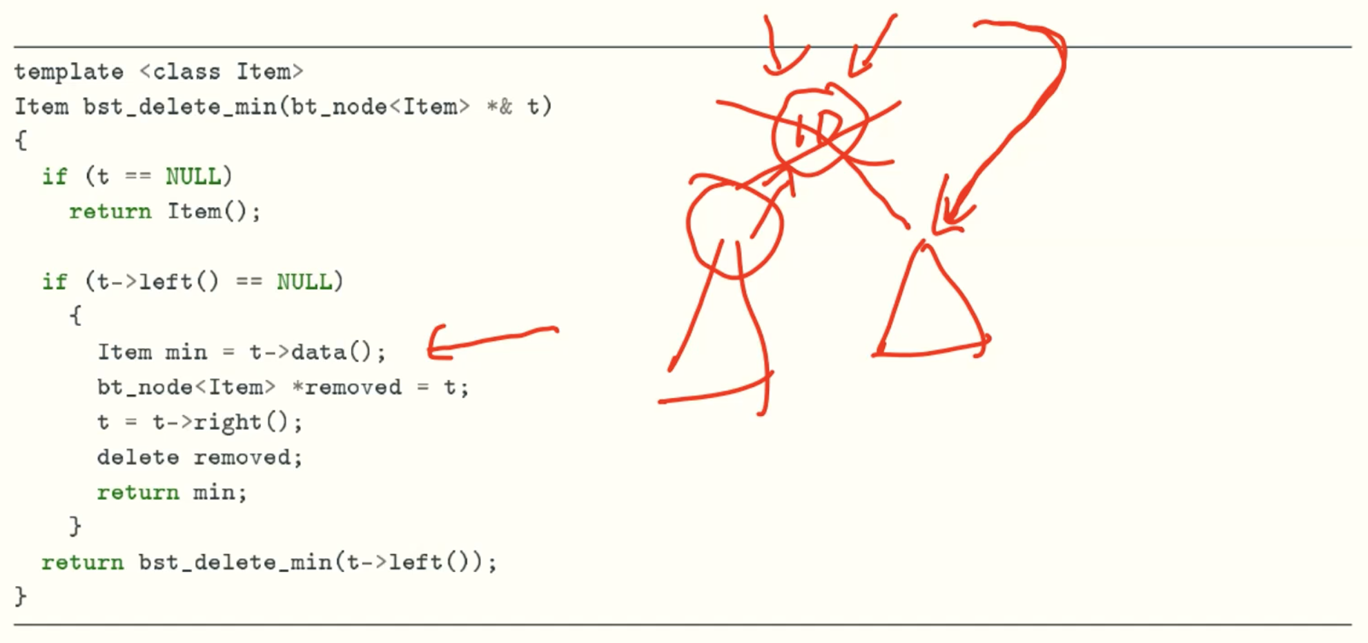
delete_min function

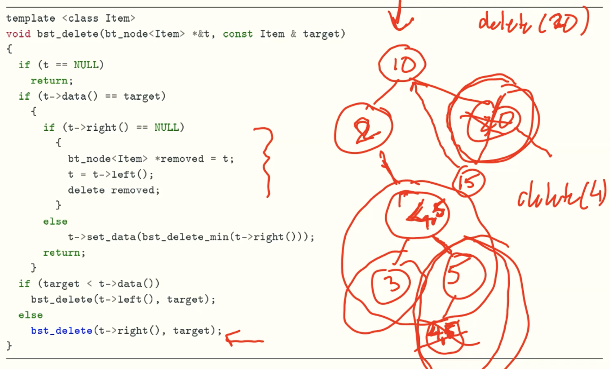
delete function

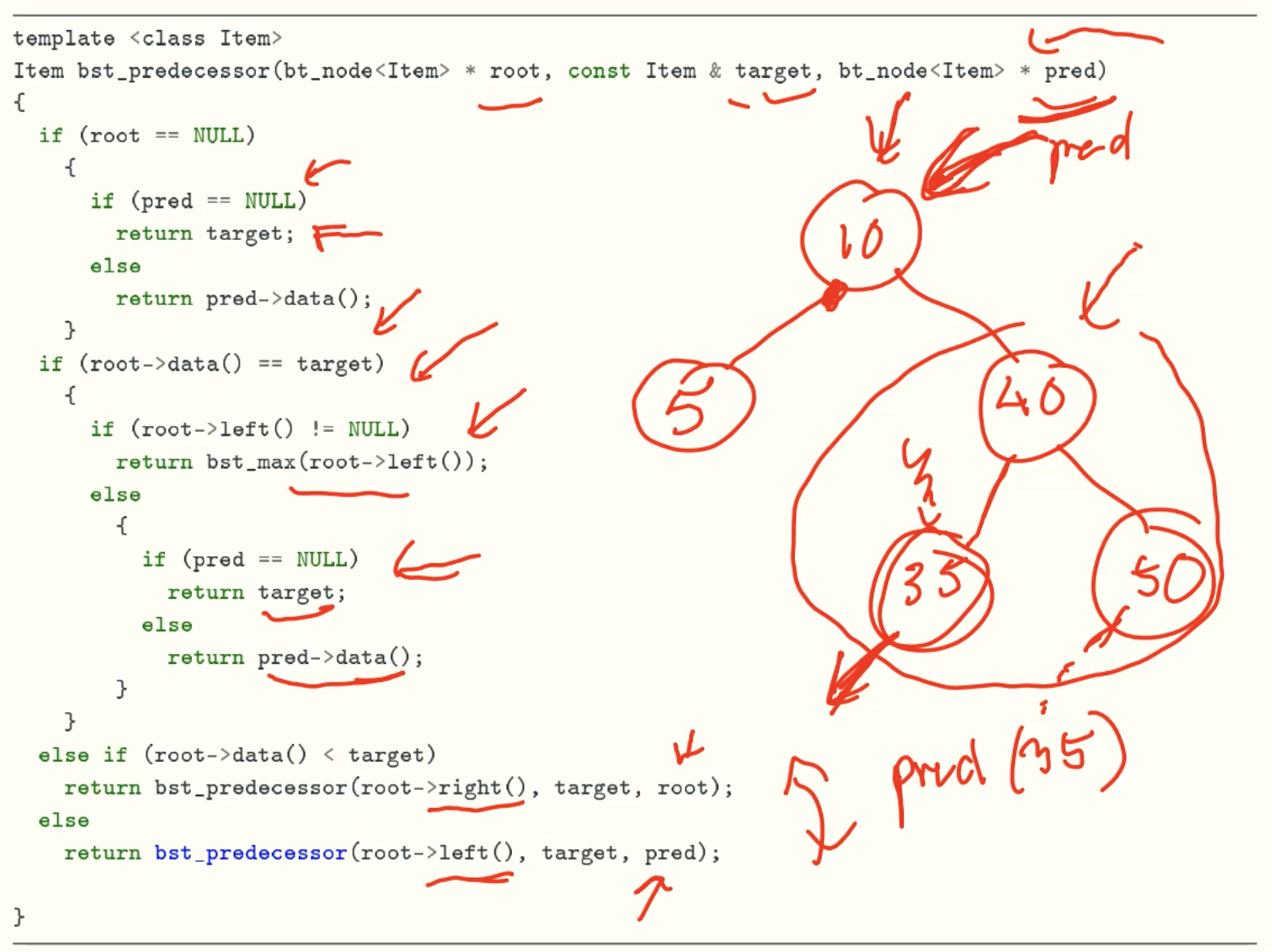
predecessor function

Example

Insert

delete

Analysis

Good average-case behavior: O(lgn) per operation.
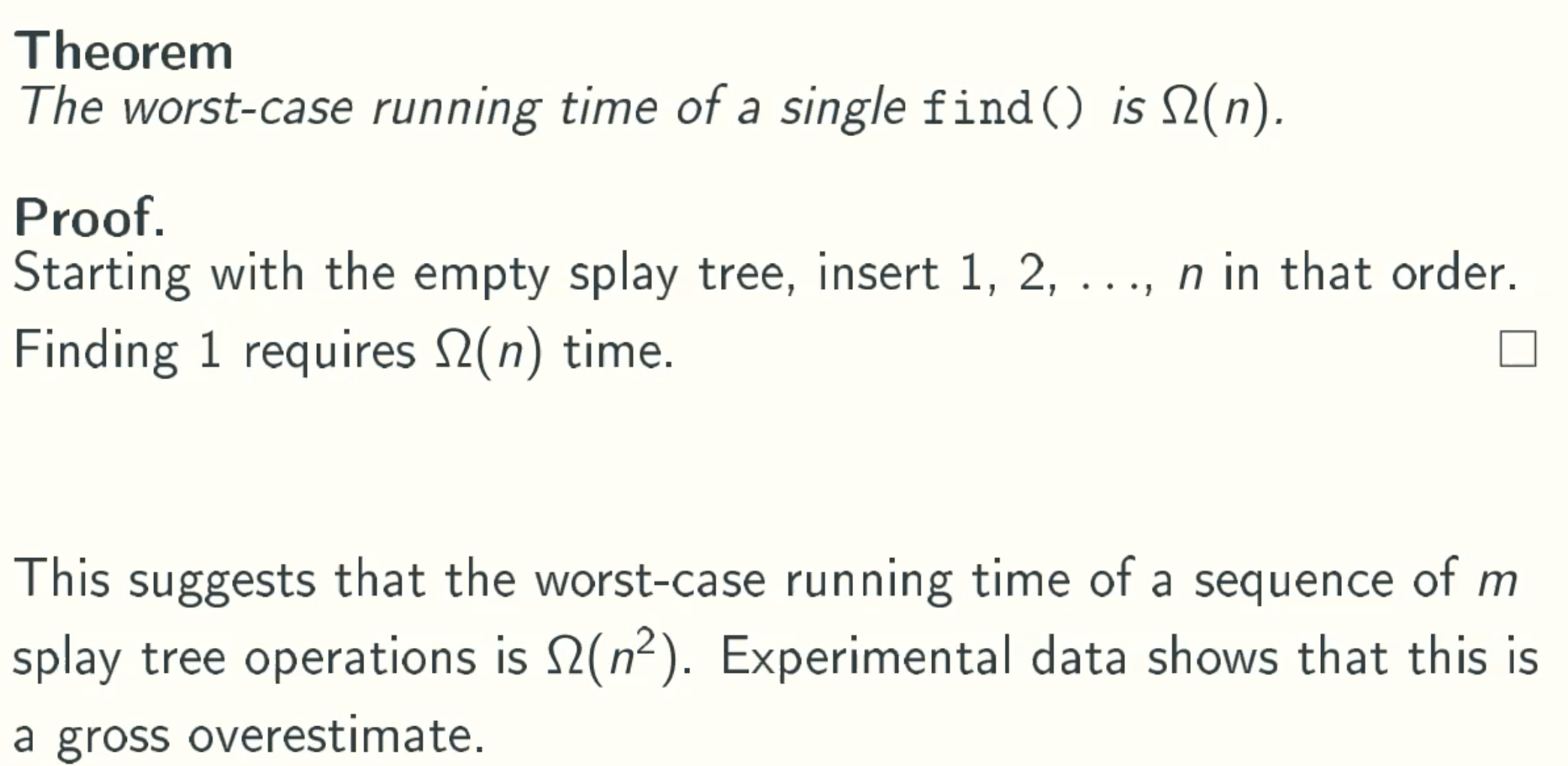
Worst-case behavior: Ω(h), where h is the height, which could be n.

Balanced BST

1. AVL trees
2. 2-3 trees(aka red-black trees)
   The worst-case running time of each operation is O(lgn)

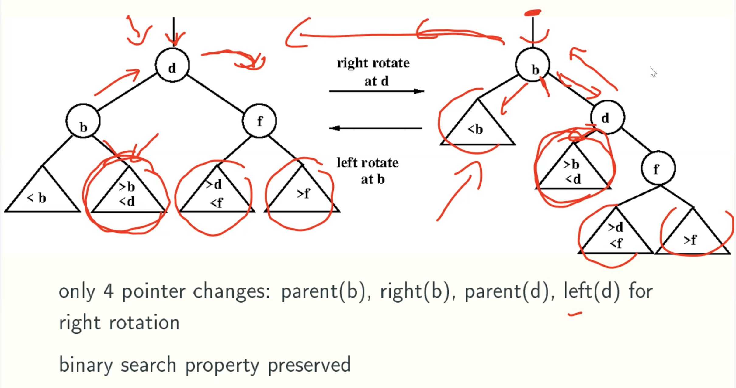
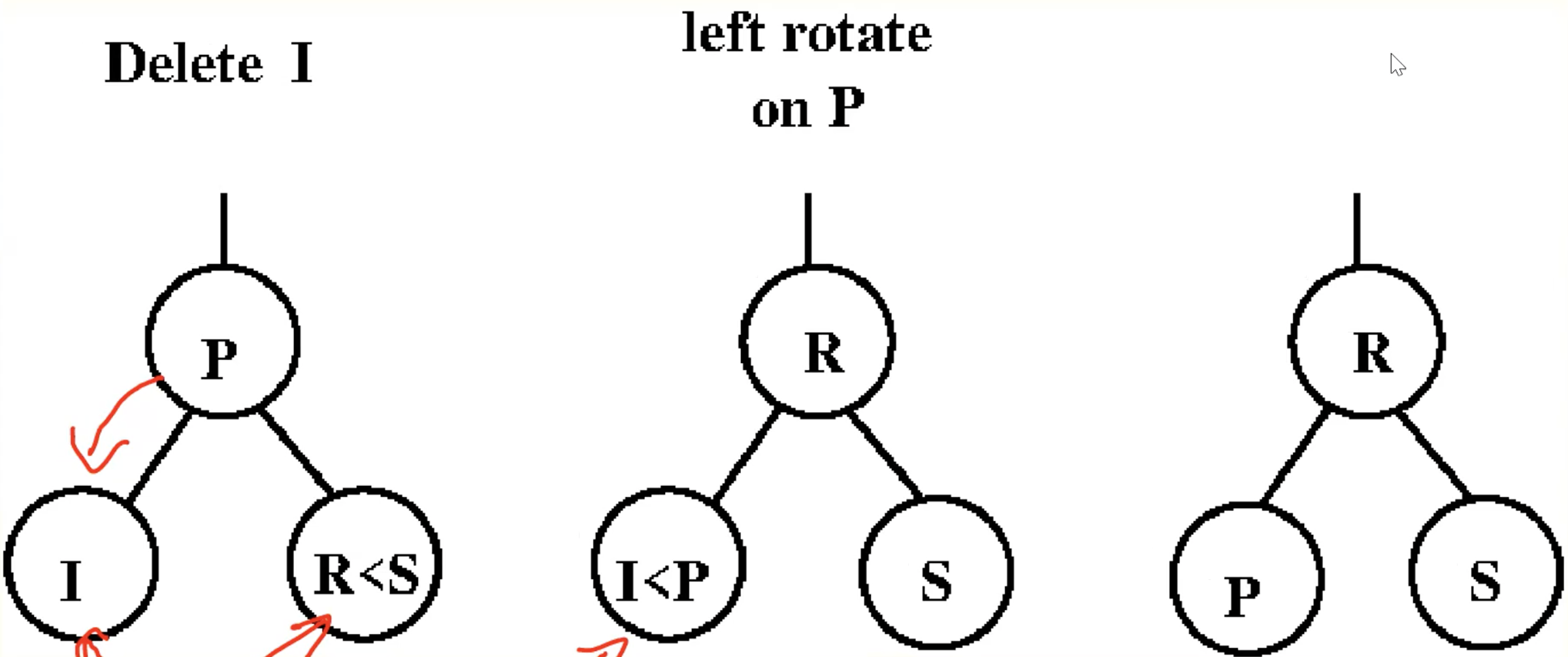
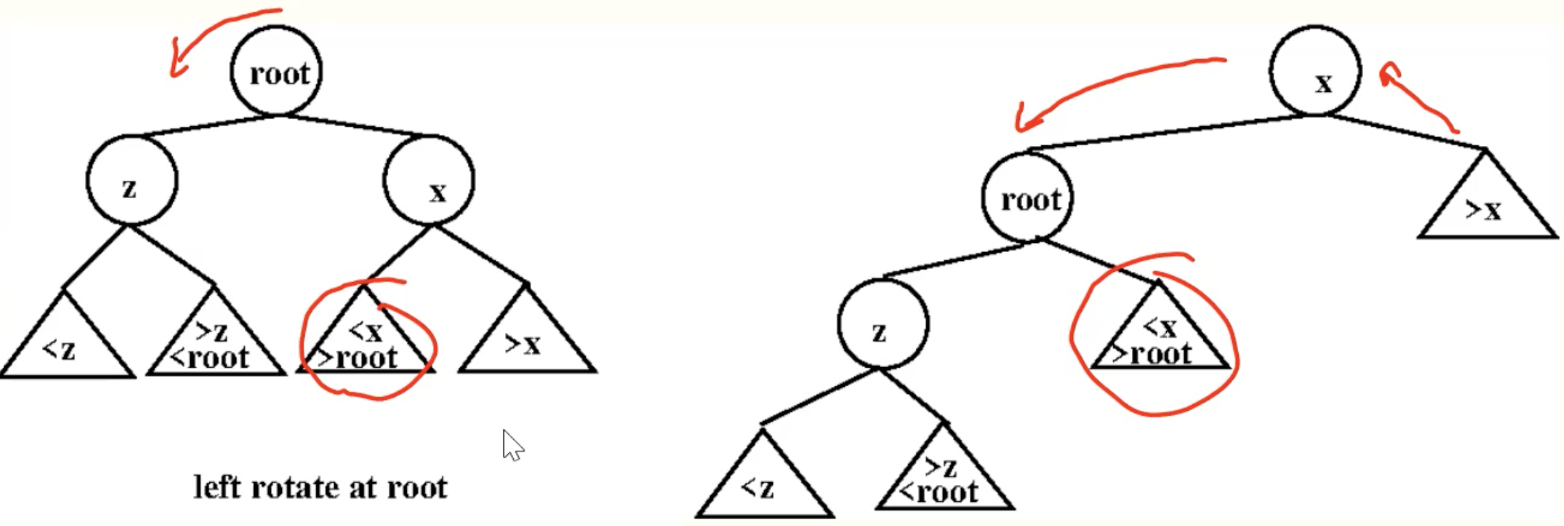
Basic Operation: rotation

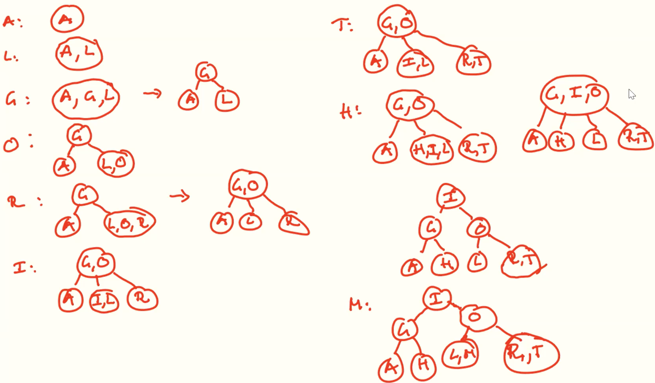
2-3 Trees

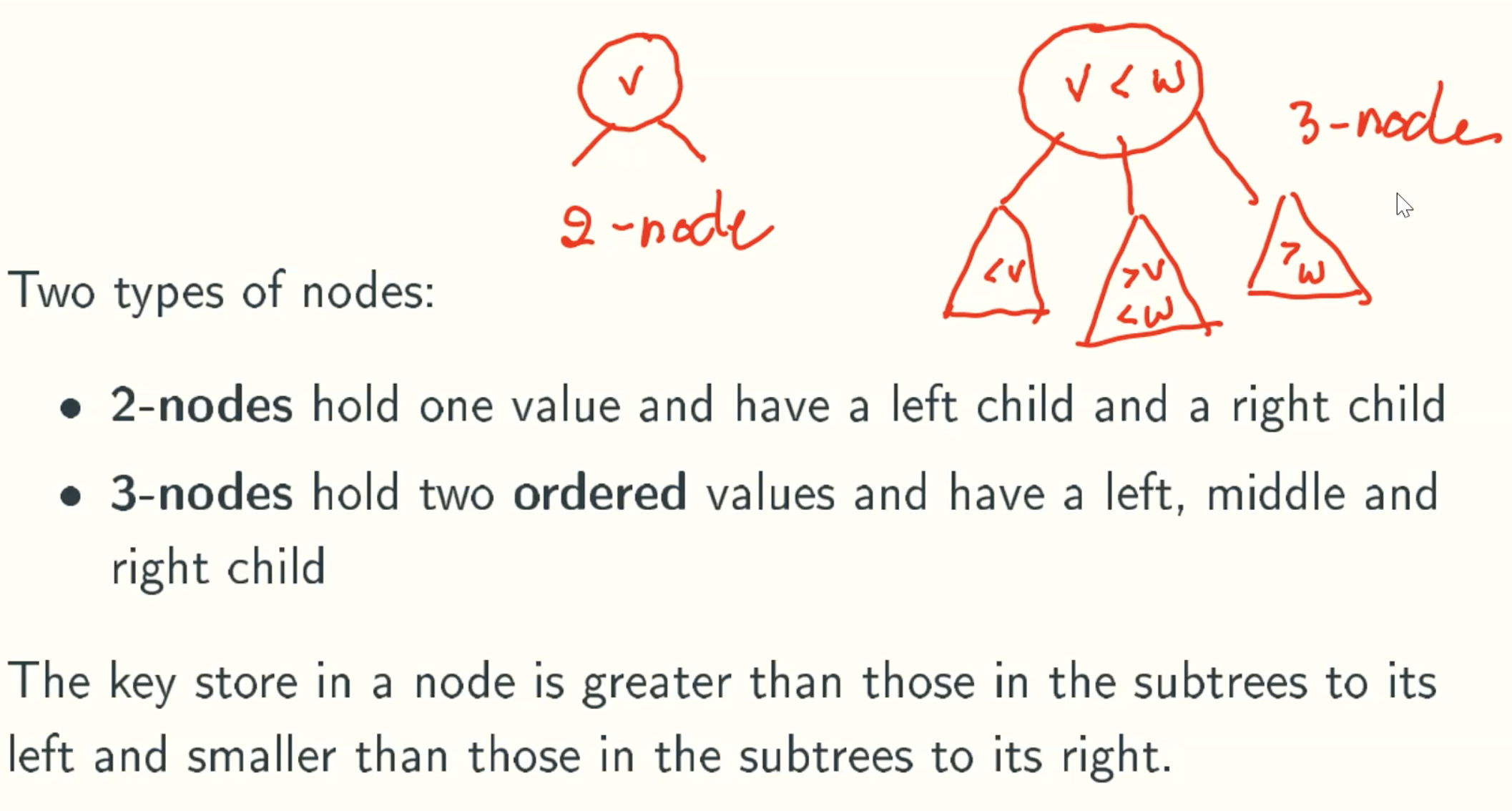
Nodes

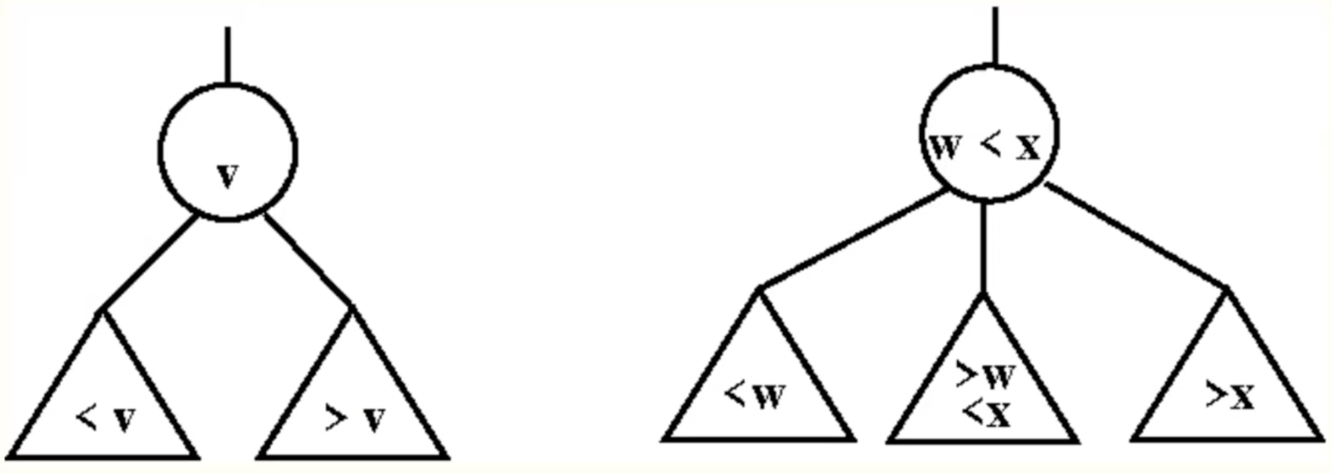
Insert

Always Insert At A Leaf

1. use binary serach property to find appropriate leaf.
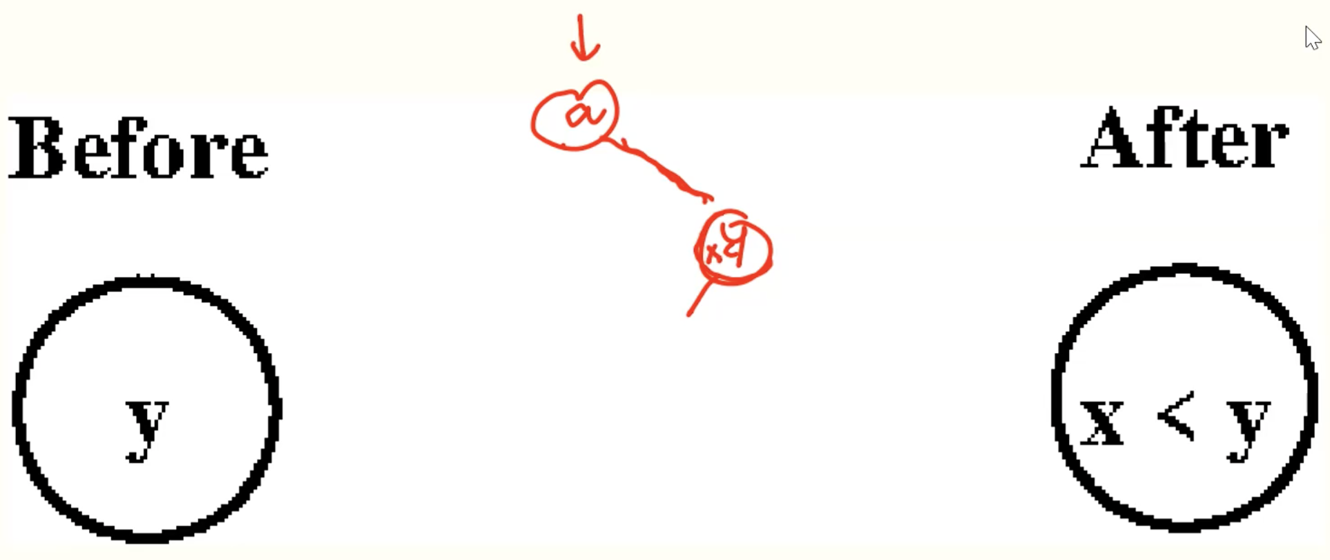
2. if leaf is a 2-node, make it a 3-node with new value.
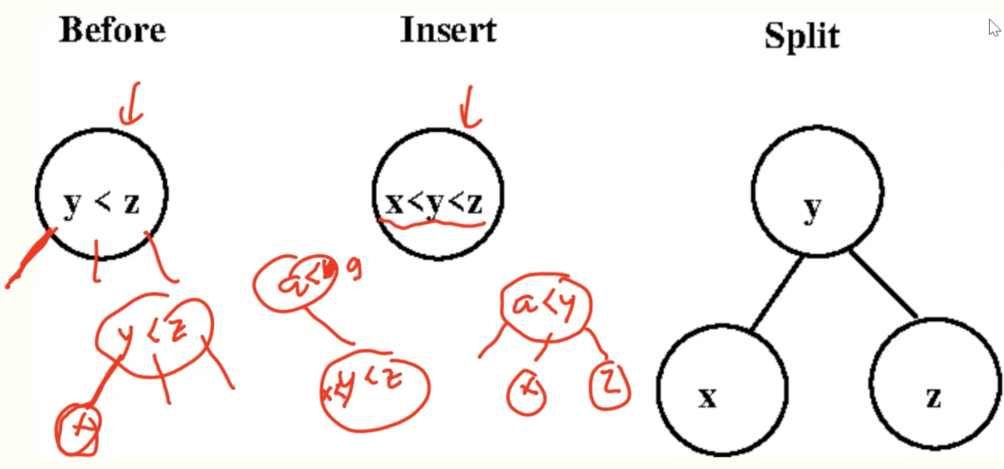
3. if leaf is a 3-node, make it a 4-node and then recursively split and insert middle value into parent node.

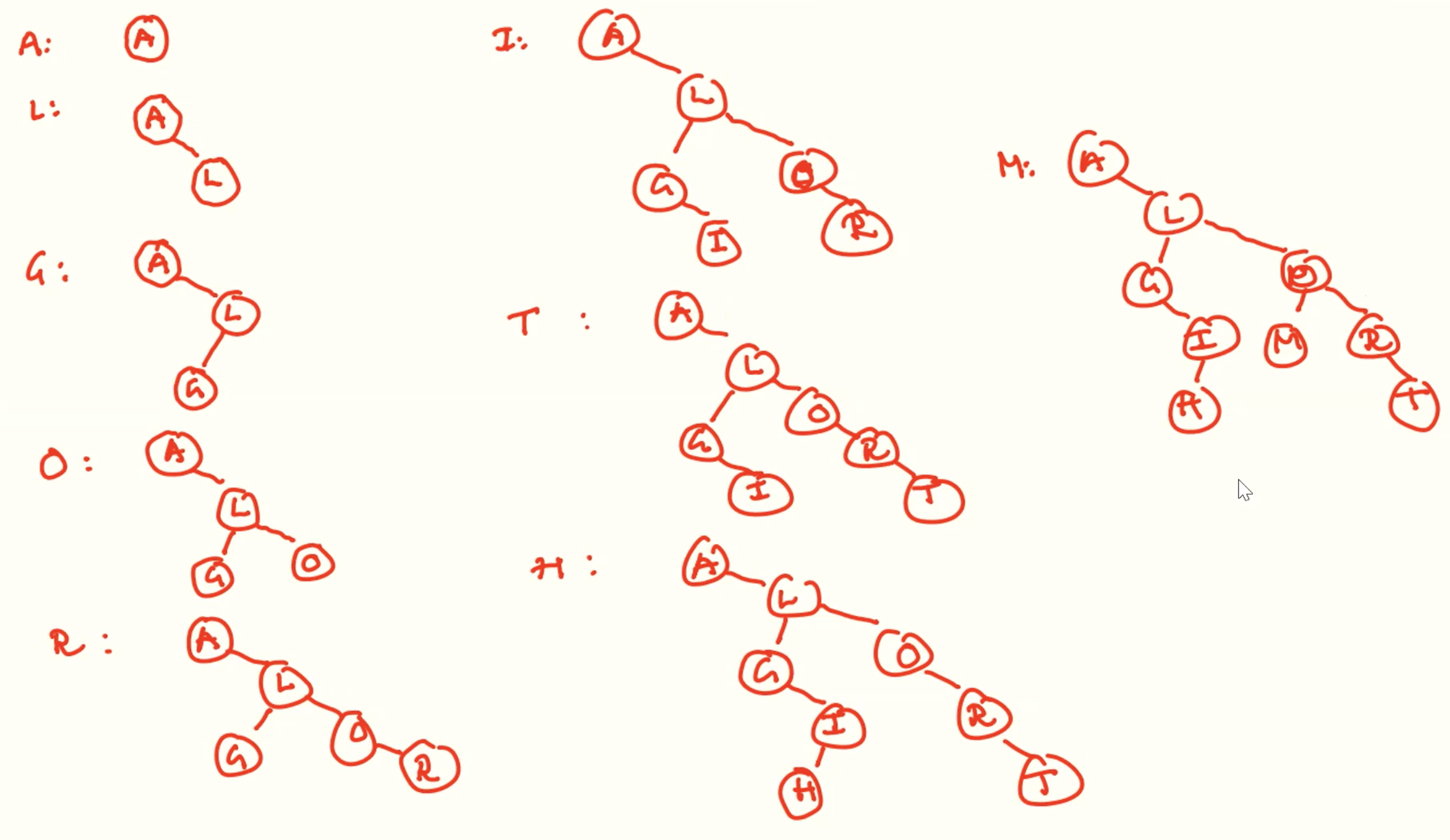
Example: inserting 2-leaf

Example: inserting 3-leaf

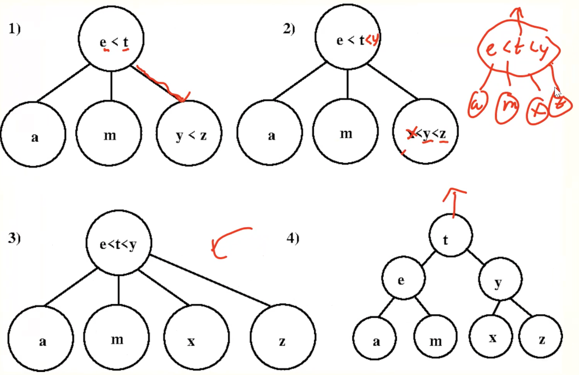
Example: inserting 3-leaf recursively

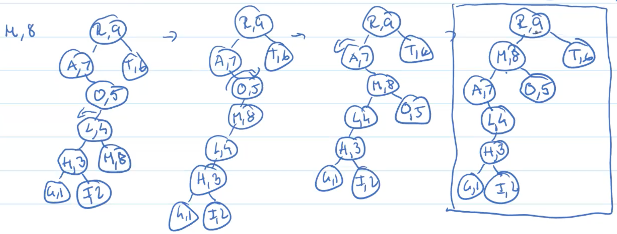
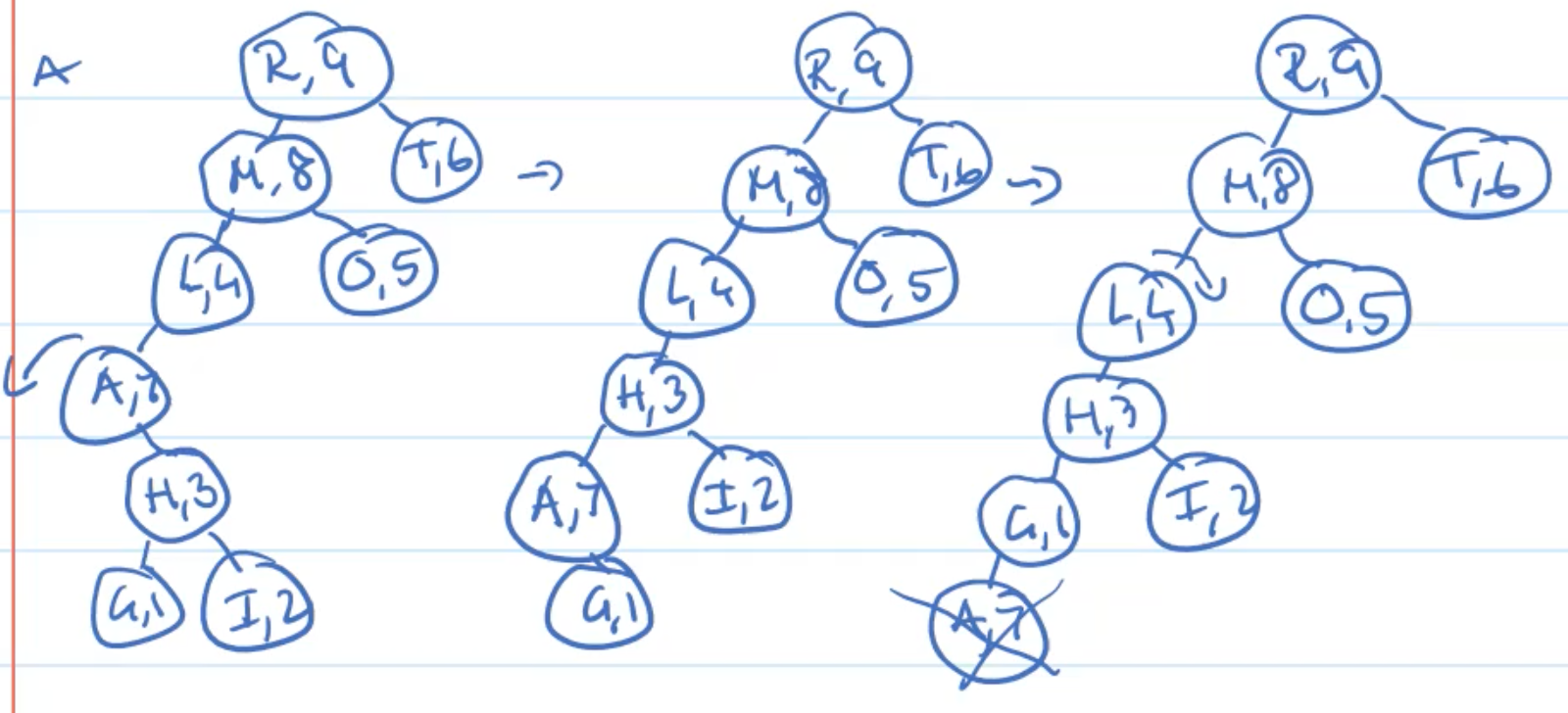
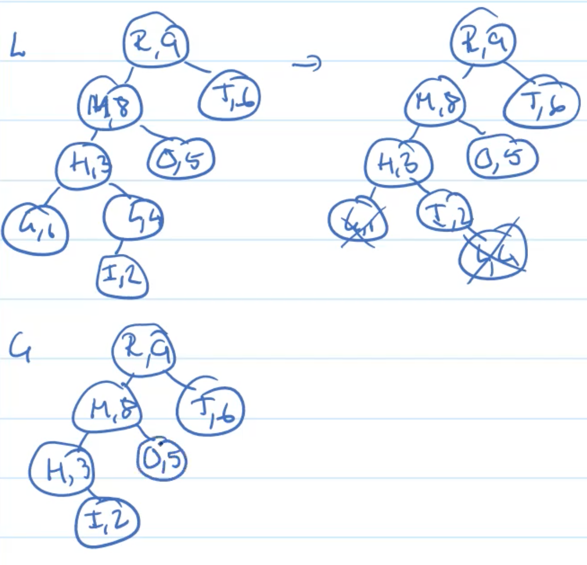
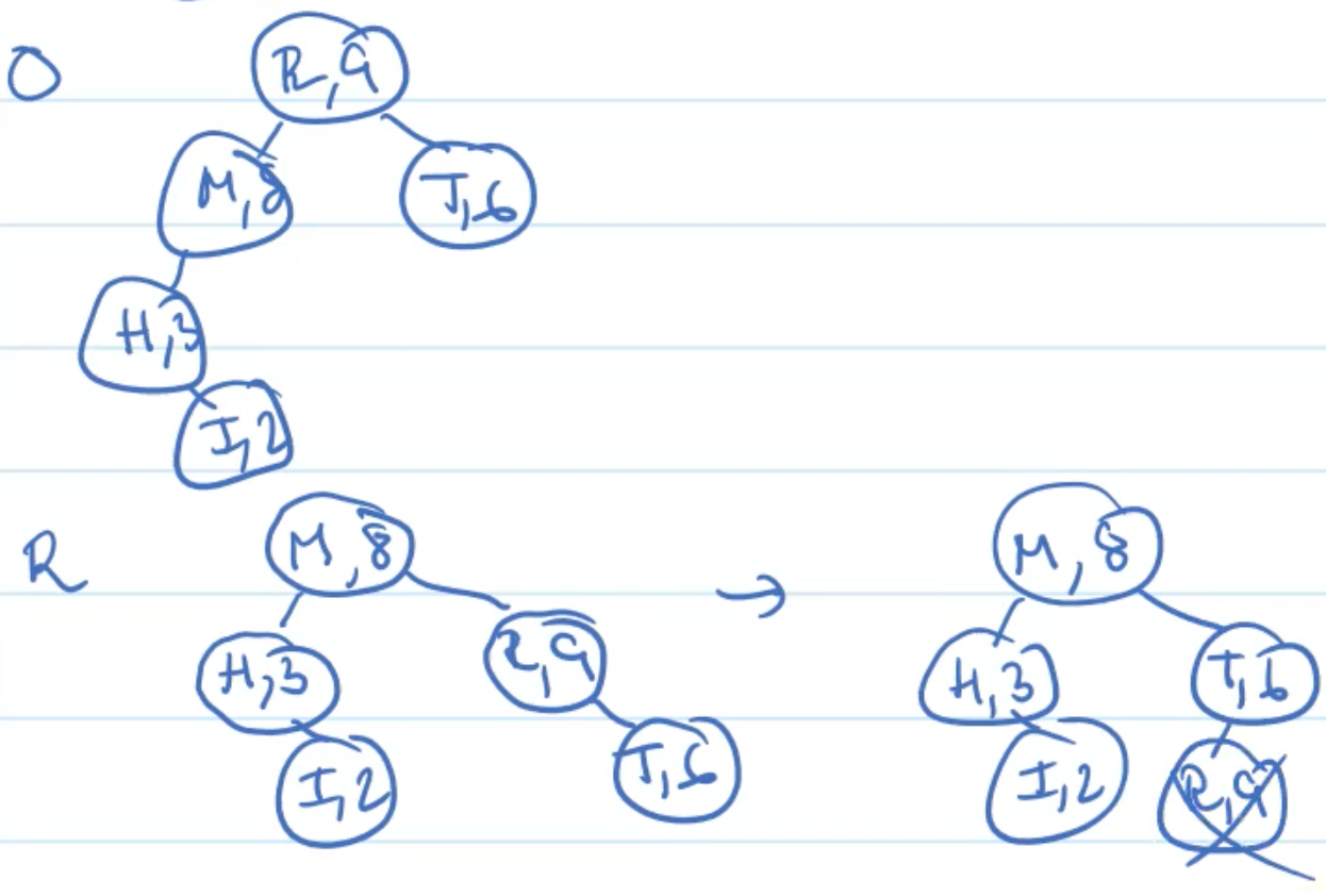
Example inserting

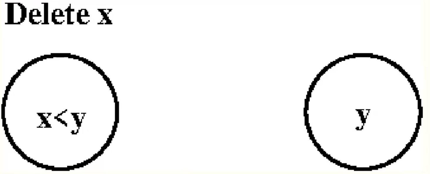
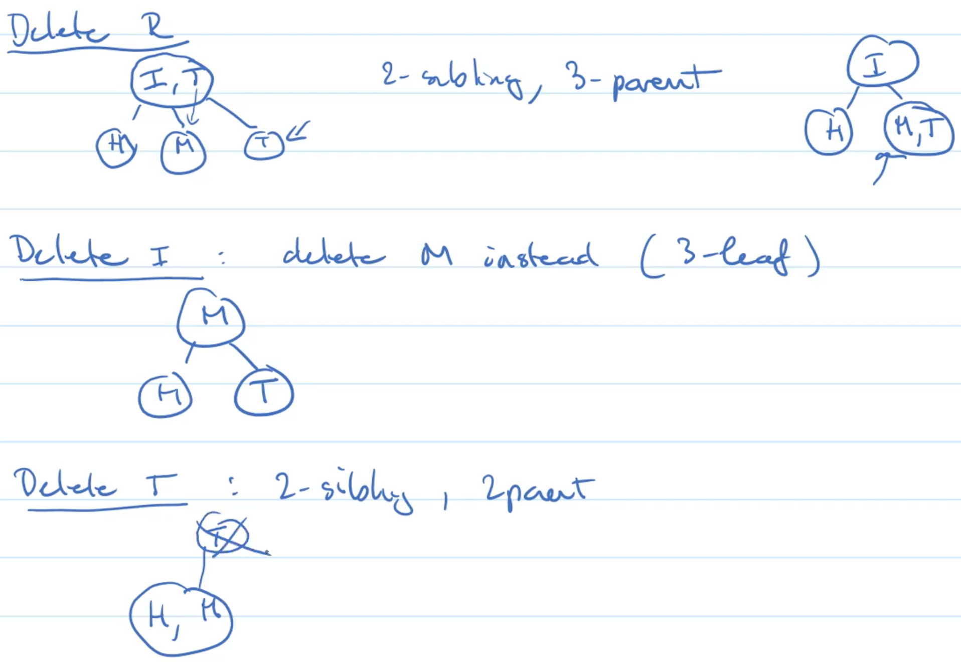
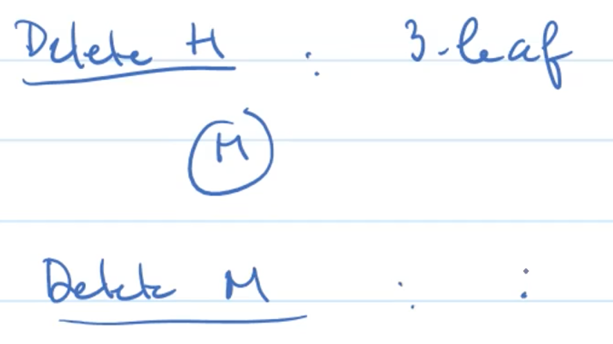
Delete

Always Delete At A Leaf

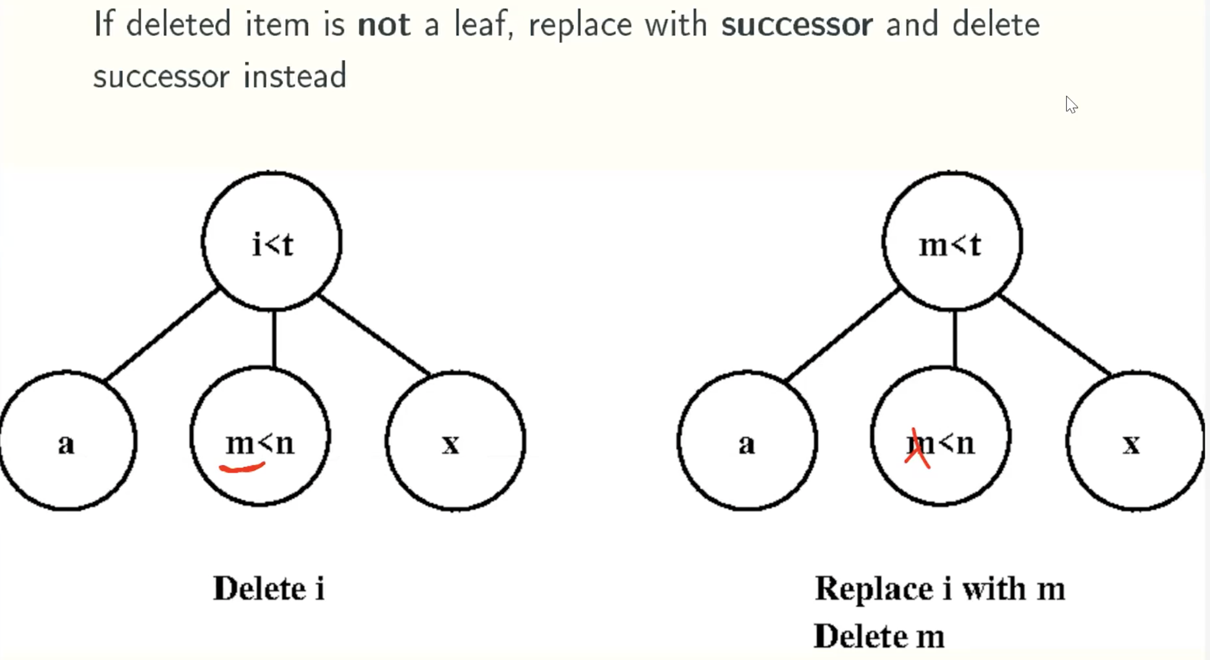
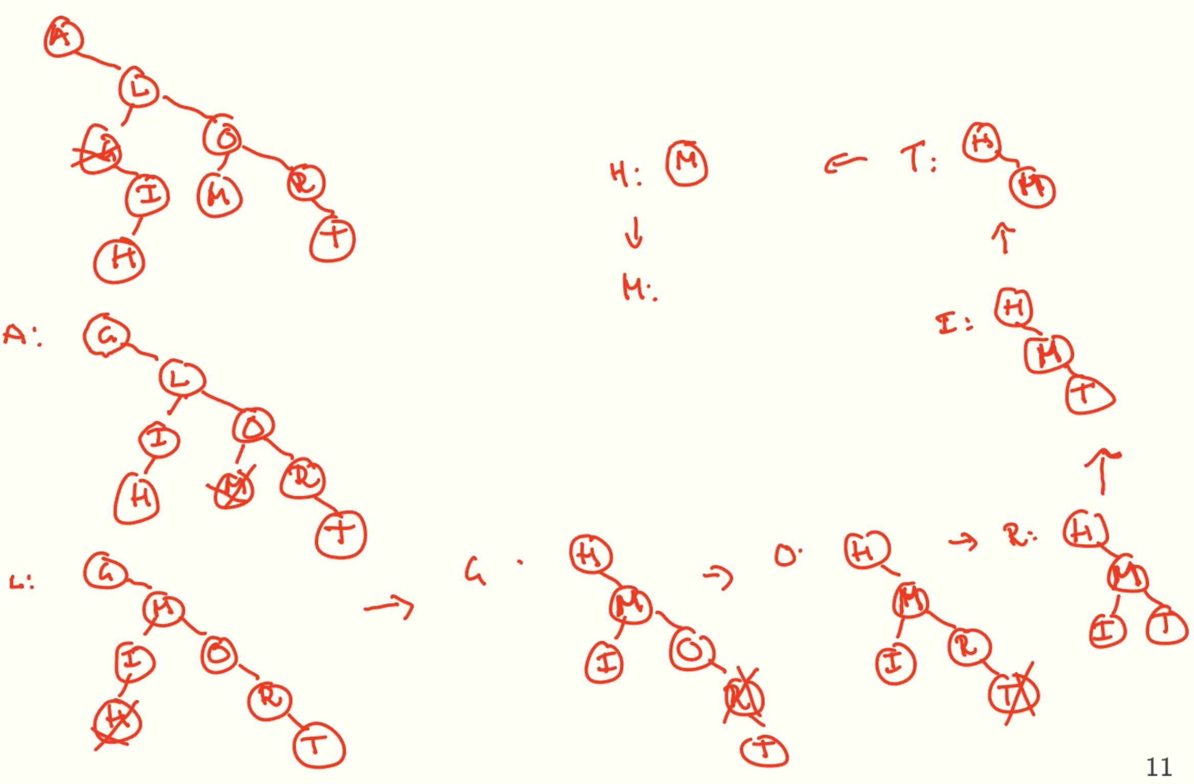
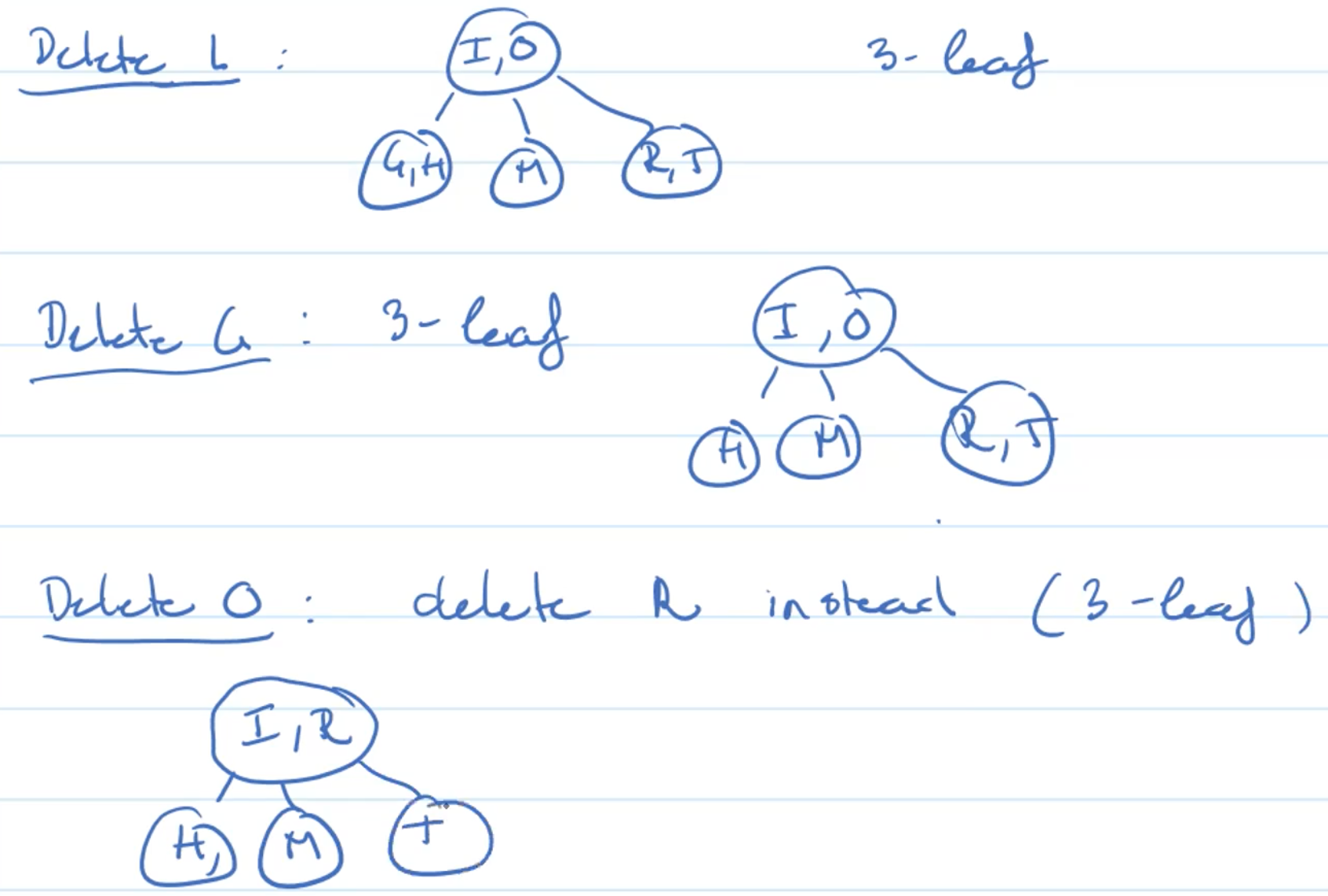
Example: delete 3-leaf

Example: 2-leaf, 3-sibling

Example: 2-leaf, 2-sibling, 3-parent

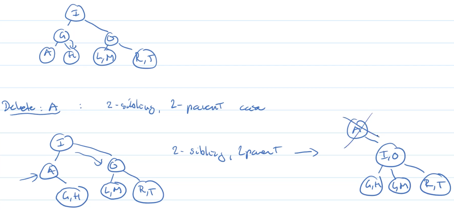
Example: 2-leaf, 2-sibling, 2-parent

Example deleting

Other Operation

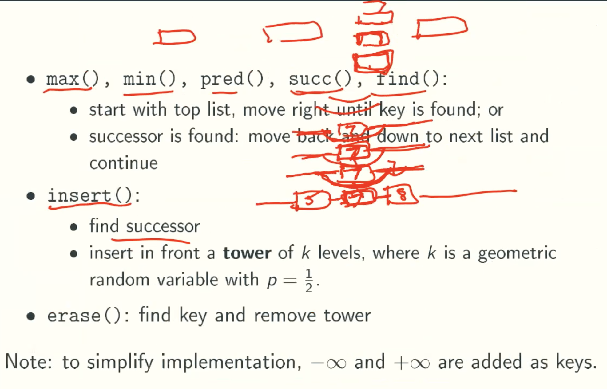
find(), min(), max(), pred() and succ() are implemented as for regular BST.

Red-Black Trees

Red-Black: Efficient Implementation Of 2-3 Trees

Red node is just a part of Black Node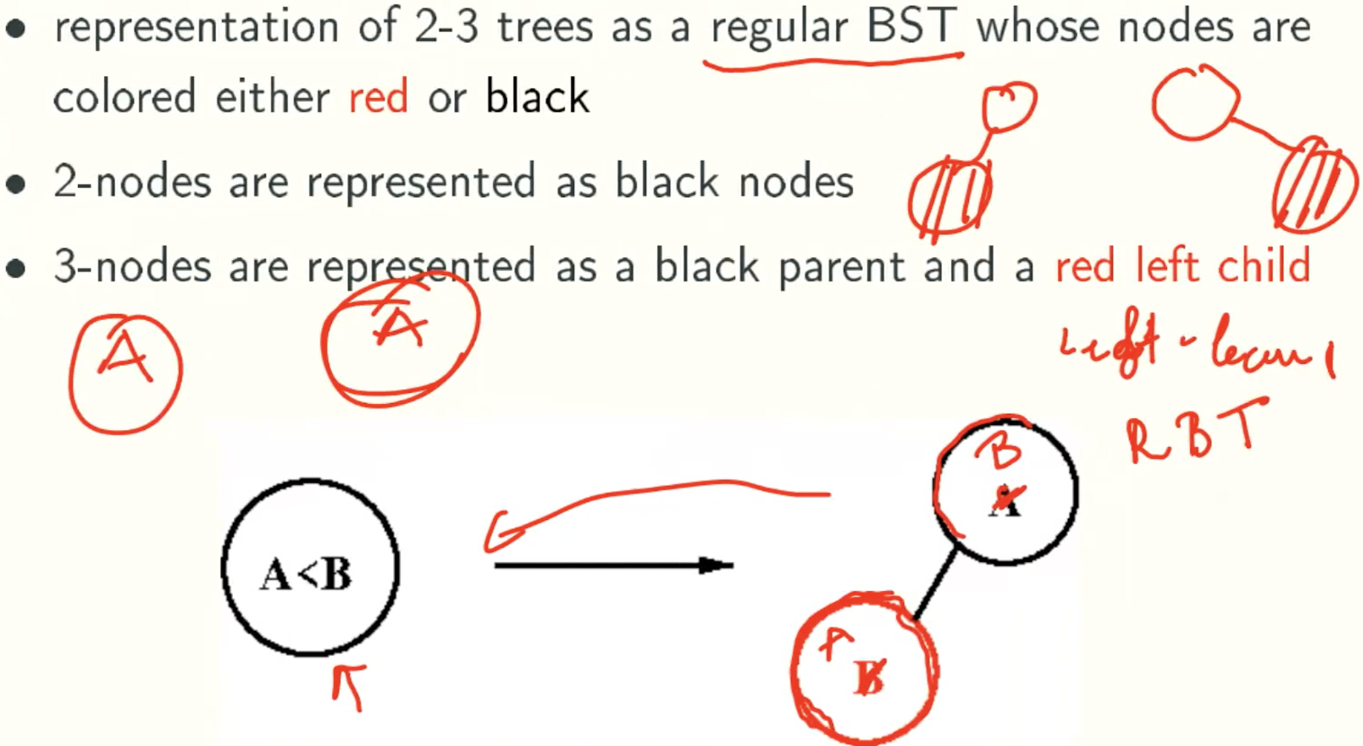

Simper Solution And Faster Balanced BST

1. treap(tree + heap): a randomized BST.
2. splay tree: an amortized BST.
3. skip list: a randomized linked list.
   details

Splay Trees

Overview

1. A variant of BST that has worst-case running time of O(mlgn) for any sequence of m BST operations, n of which are insertions.
2. Each regular BST operation is followed by a splay operation, which moves the most recently accessed element to the root.

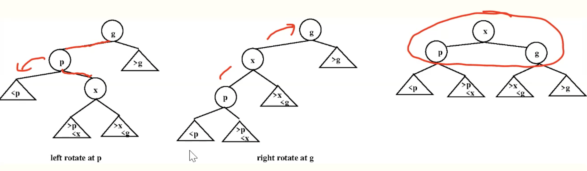
Splay Operation

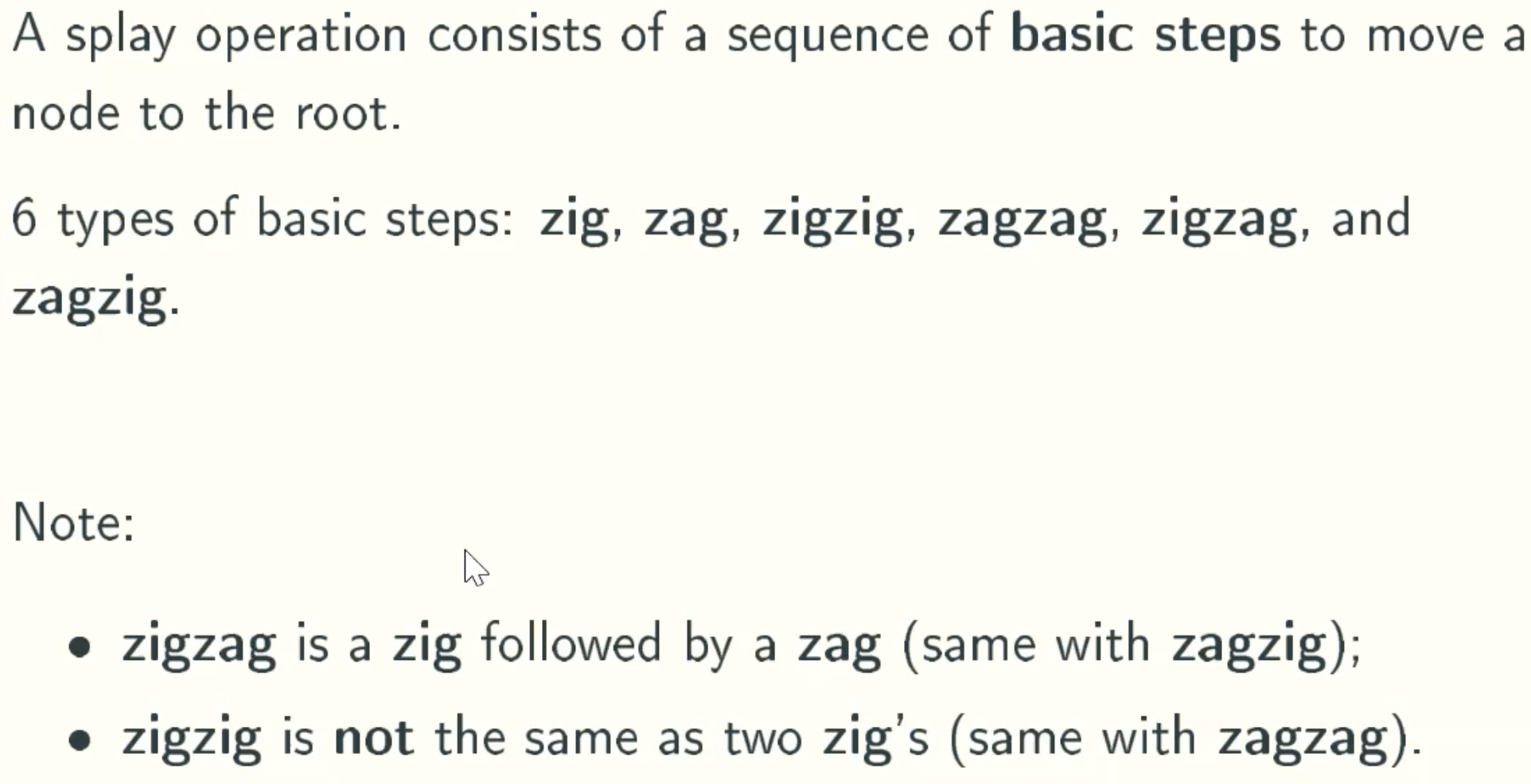
Basic Step

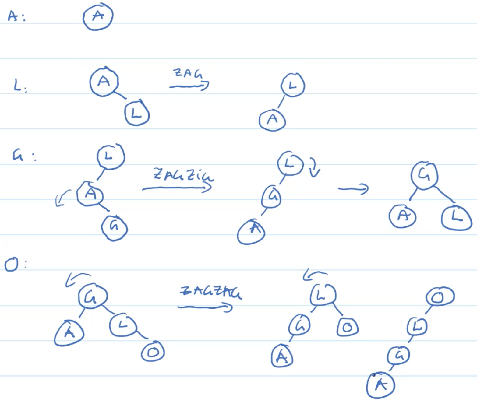
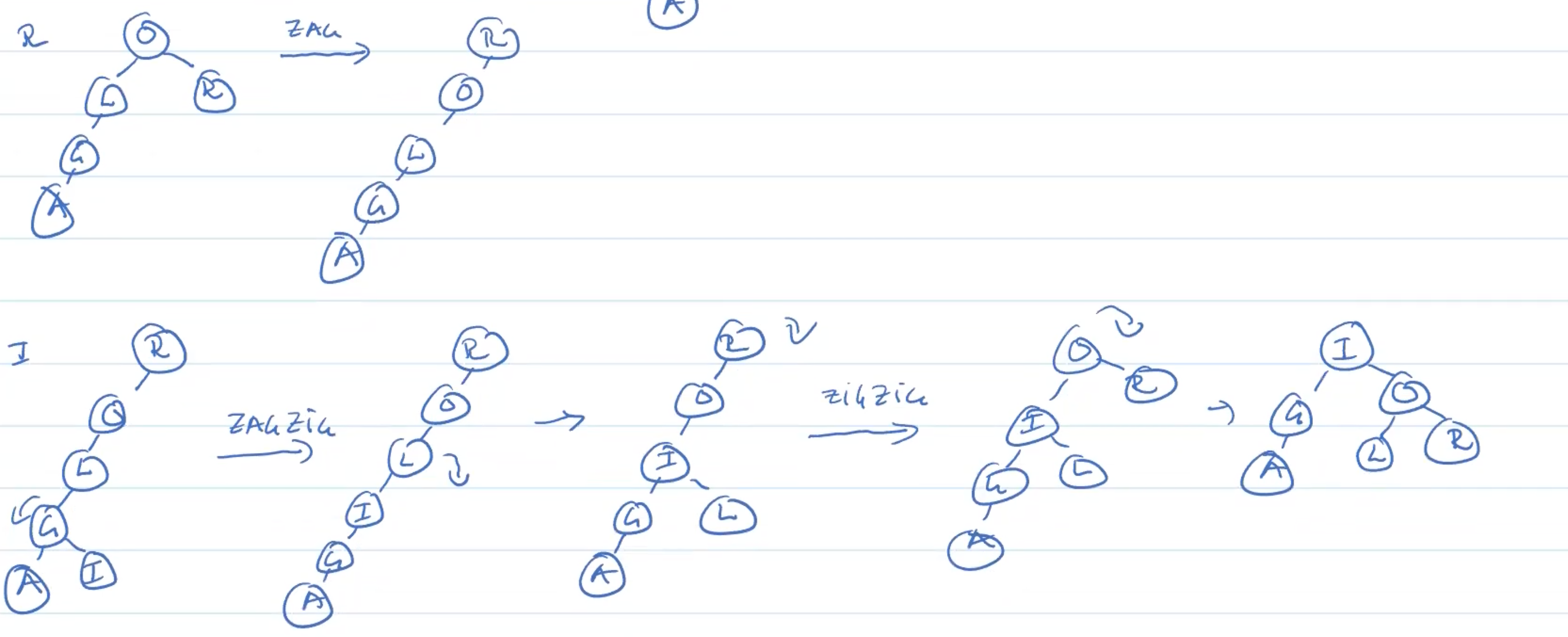
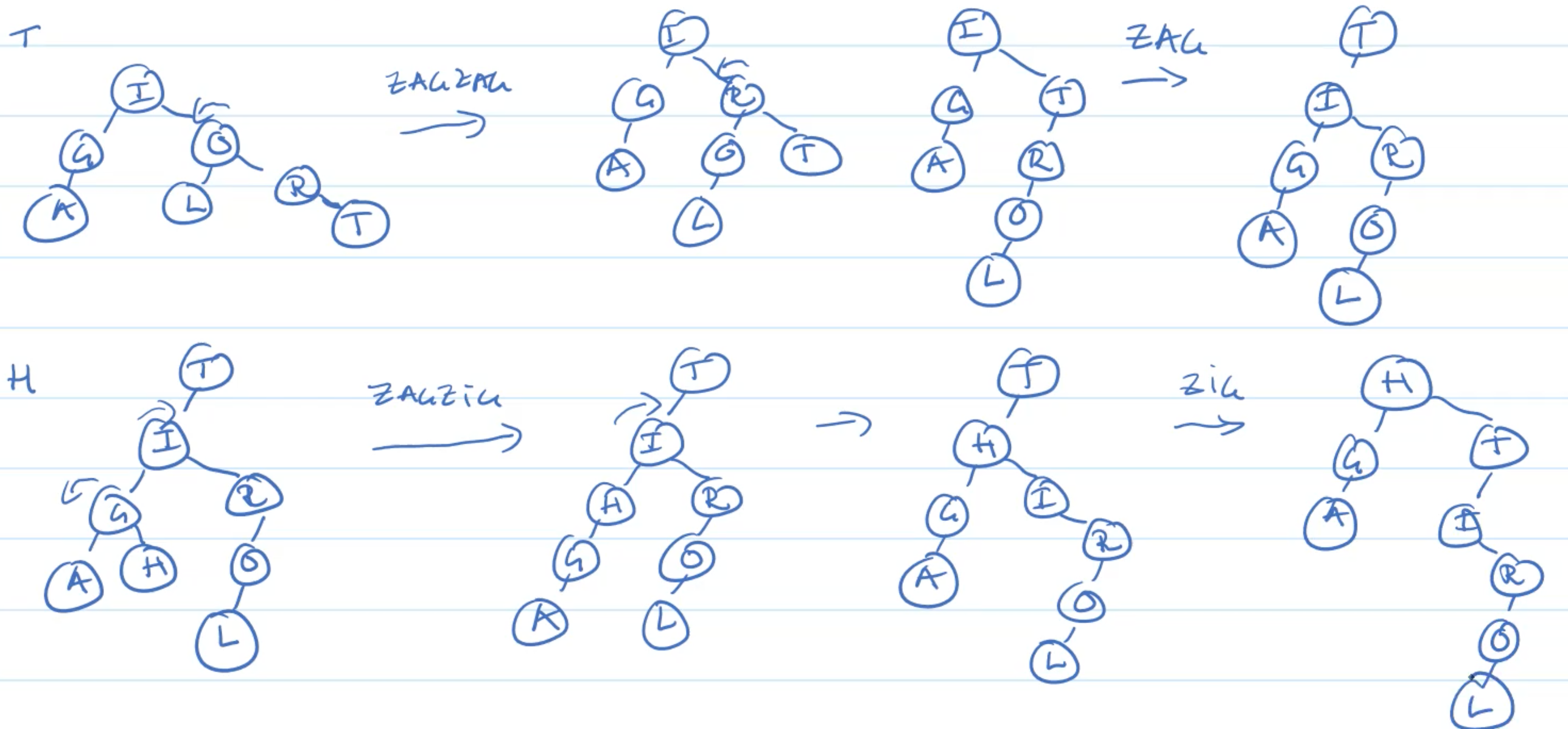
Zig

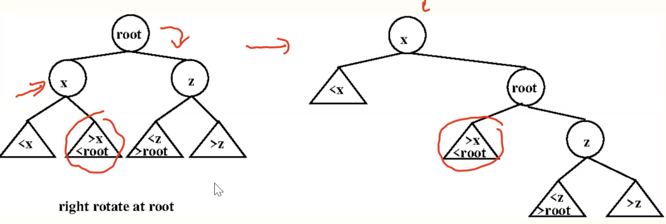
Zag

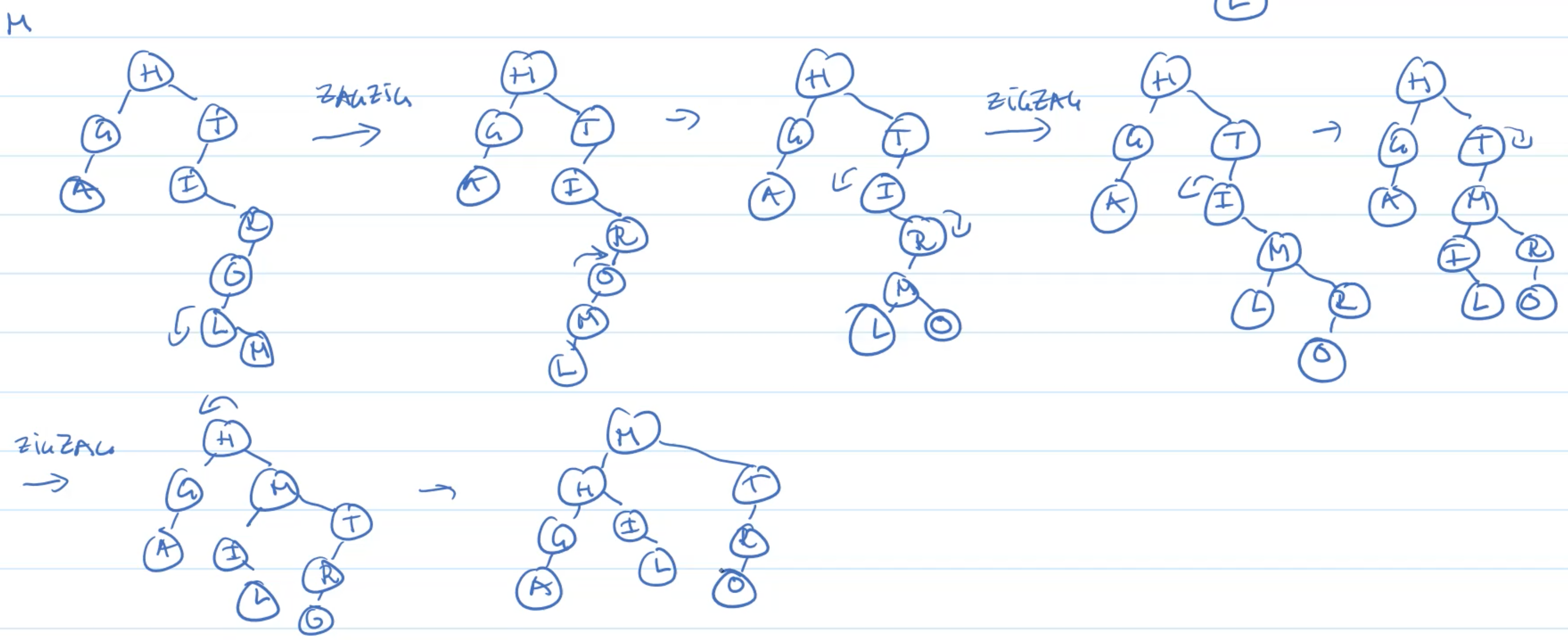
ZigZig

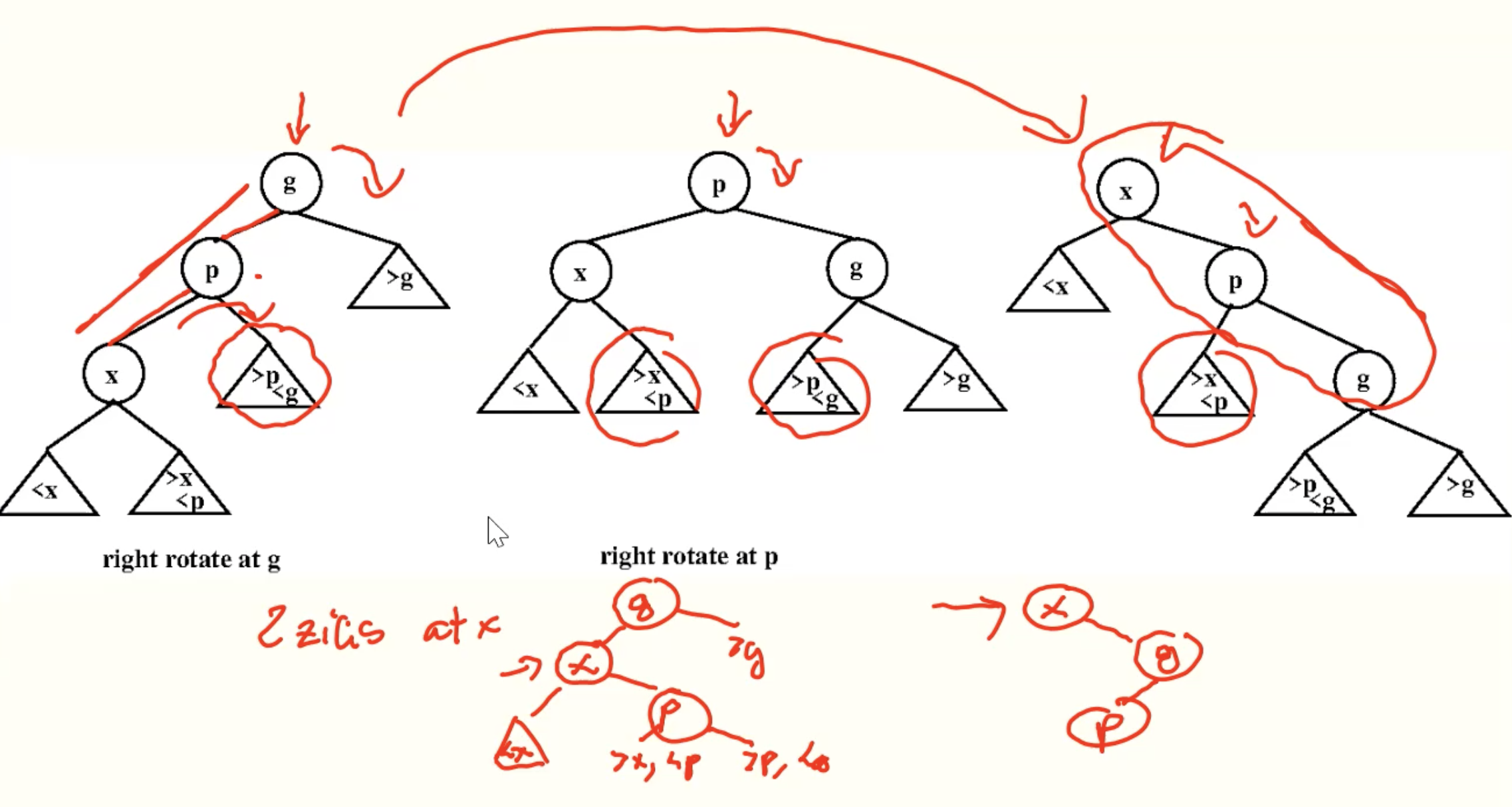
ZagZag

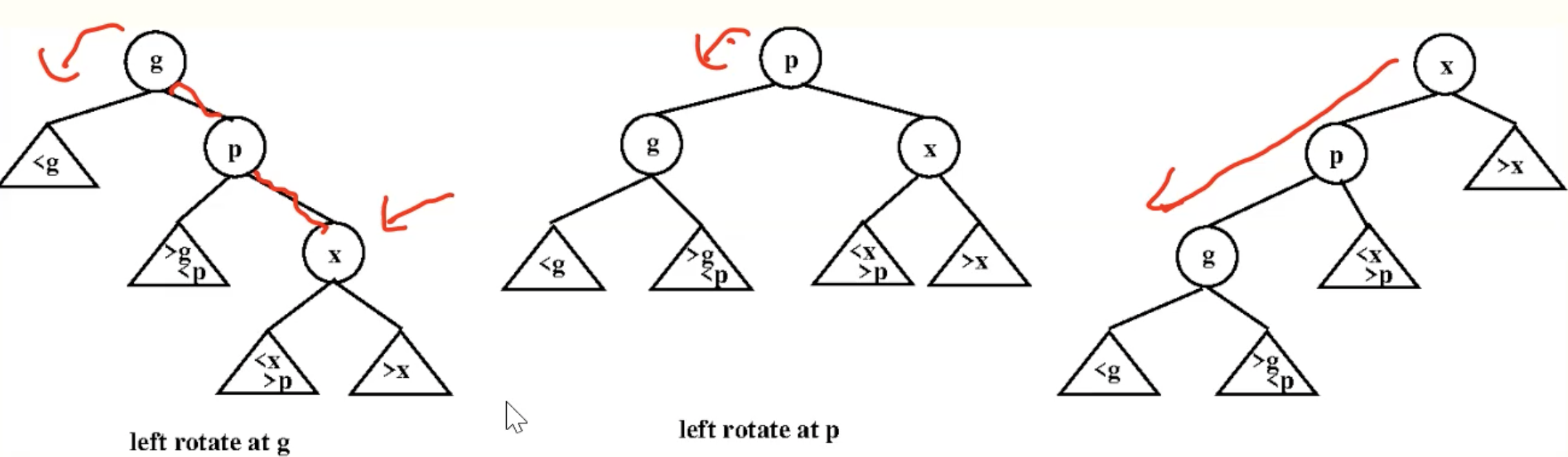
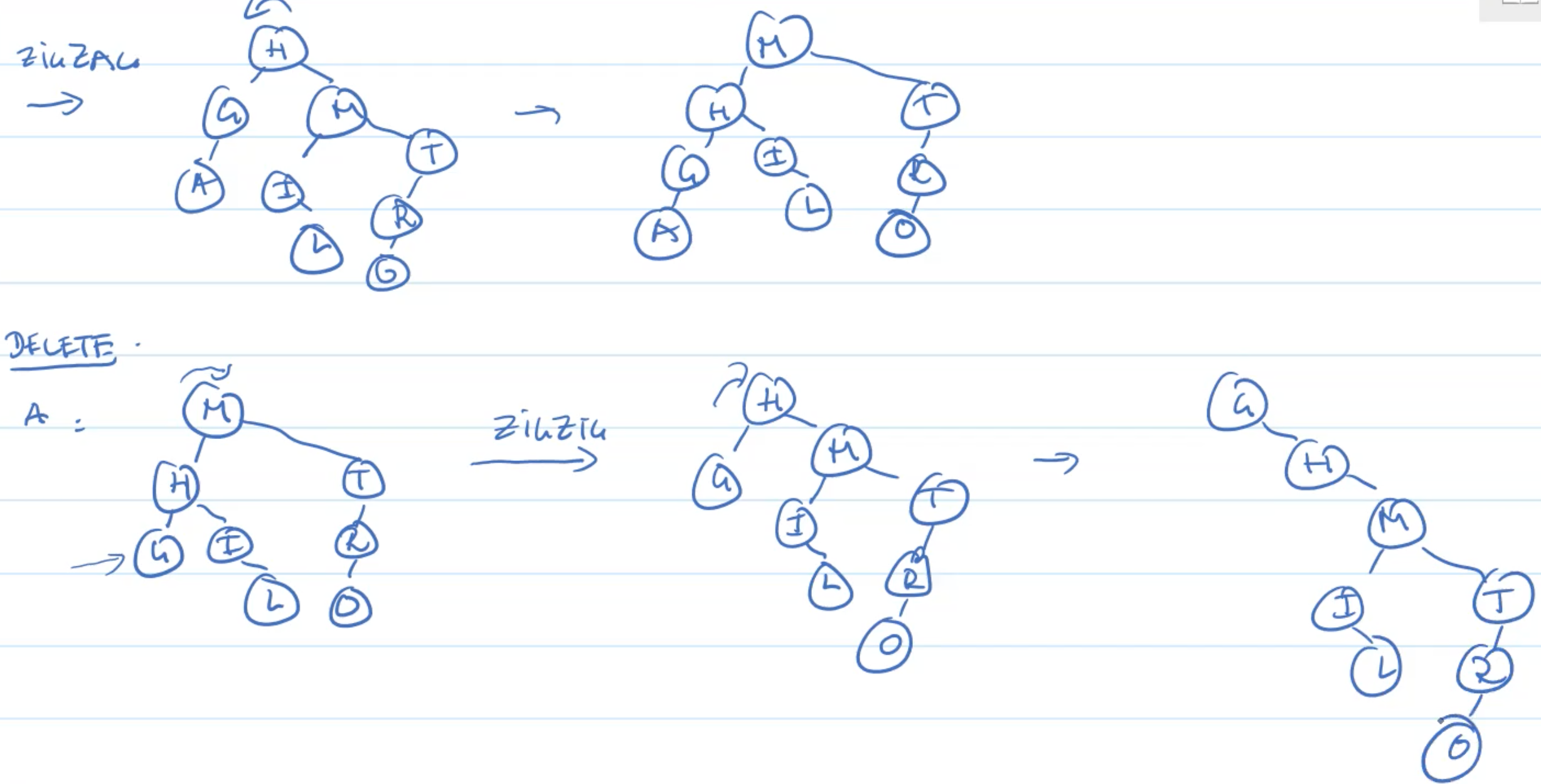
ZigZag

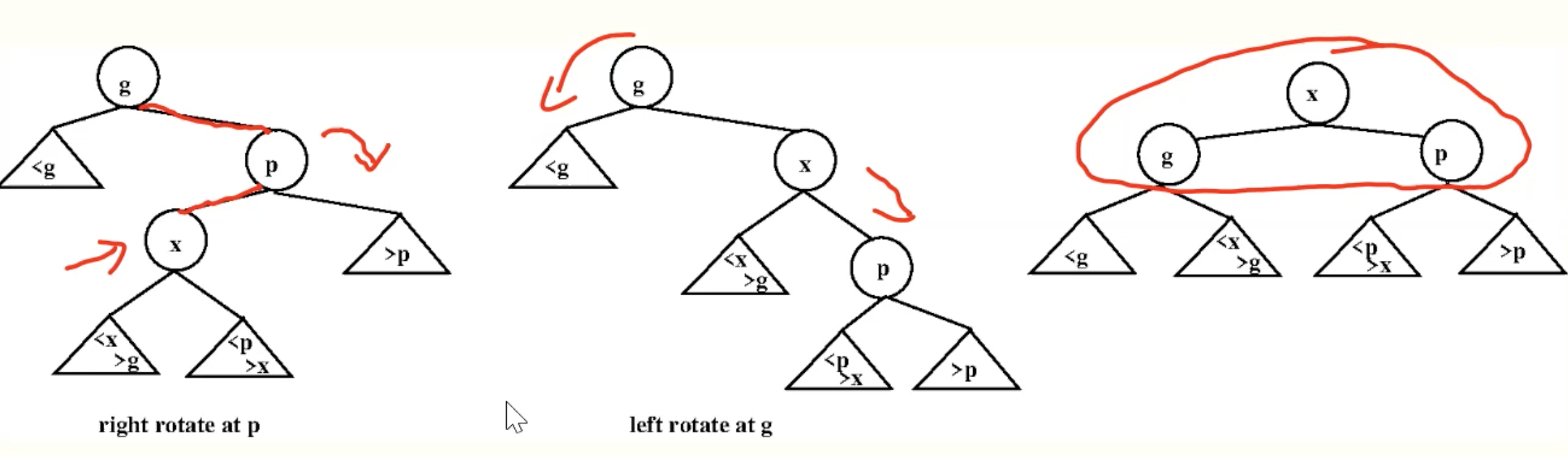
ZagZig

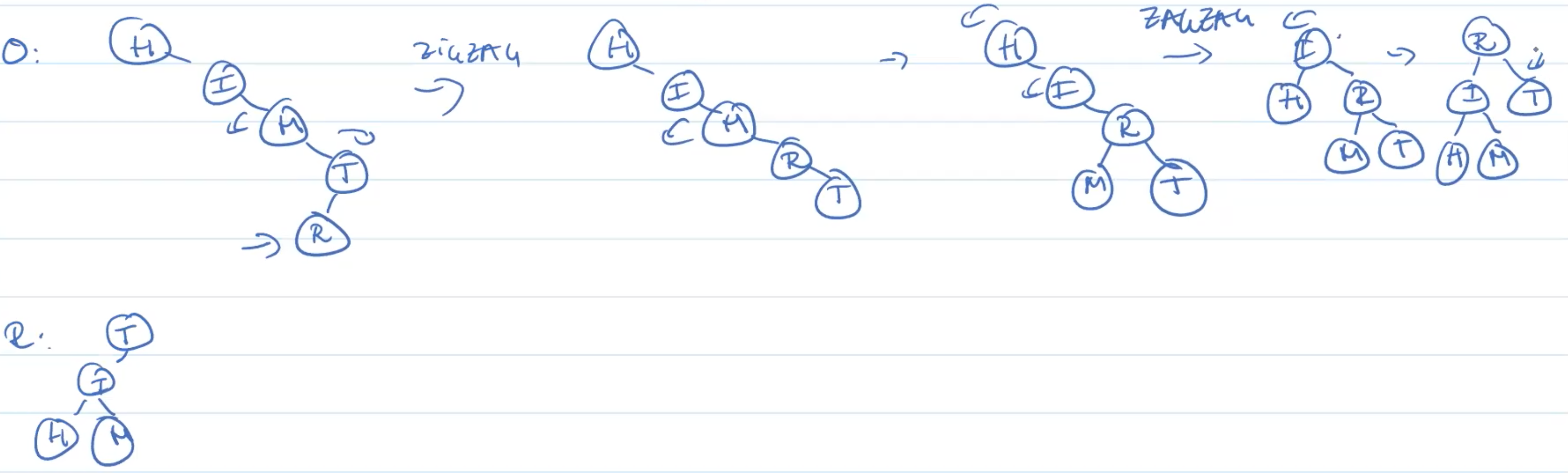
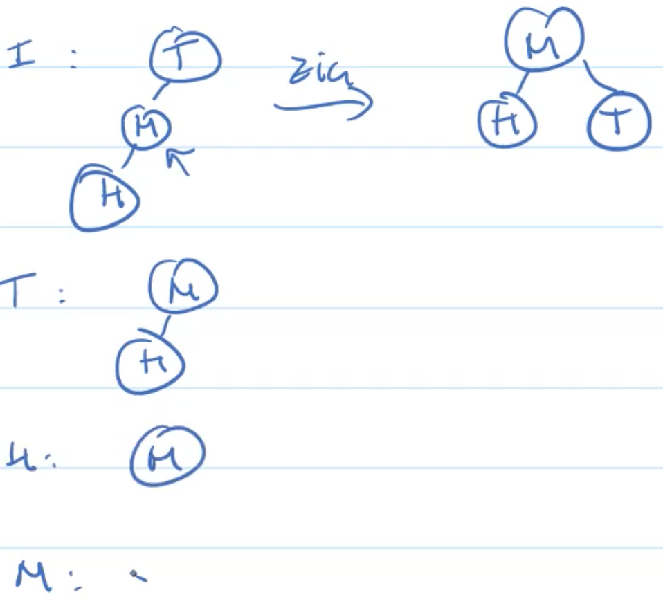
Example: Insertion

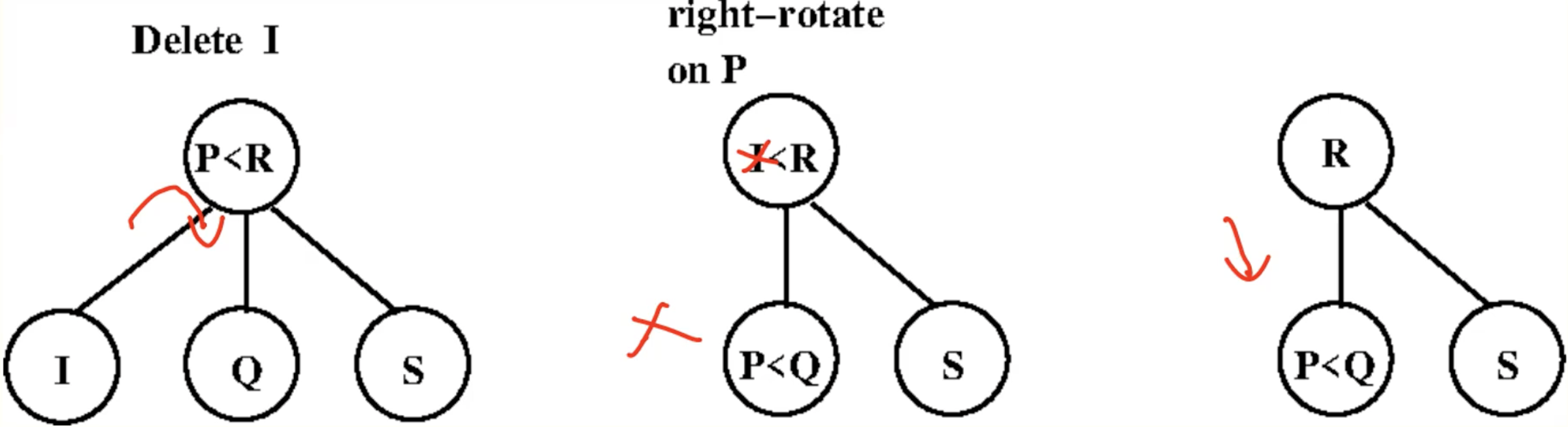
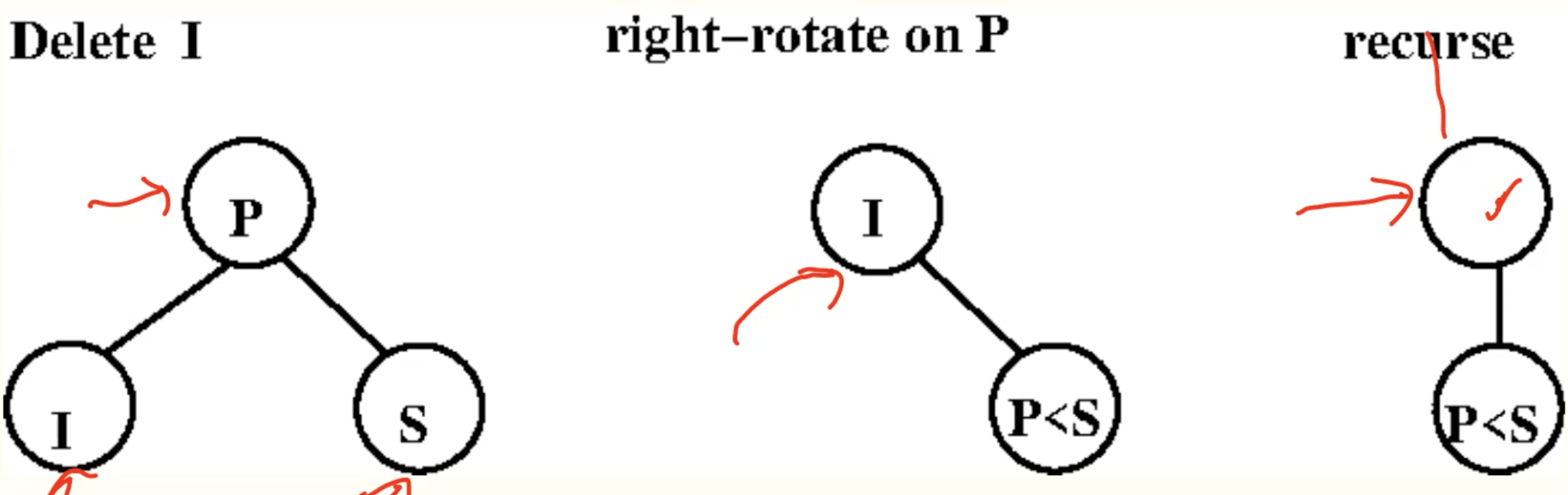
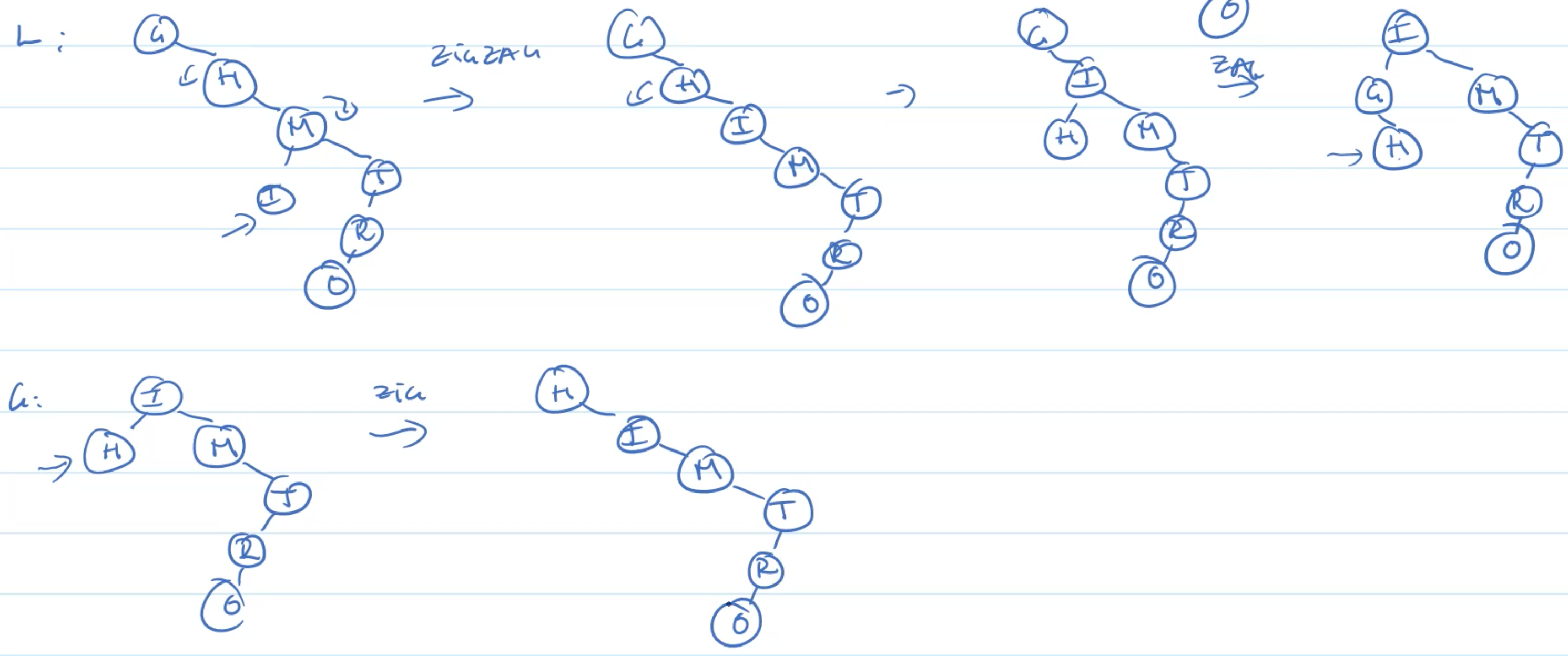
Example: Deletion

Normal Analysis

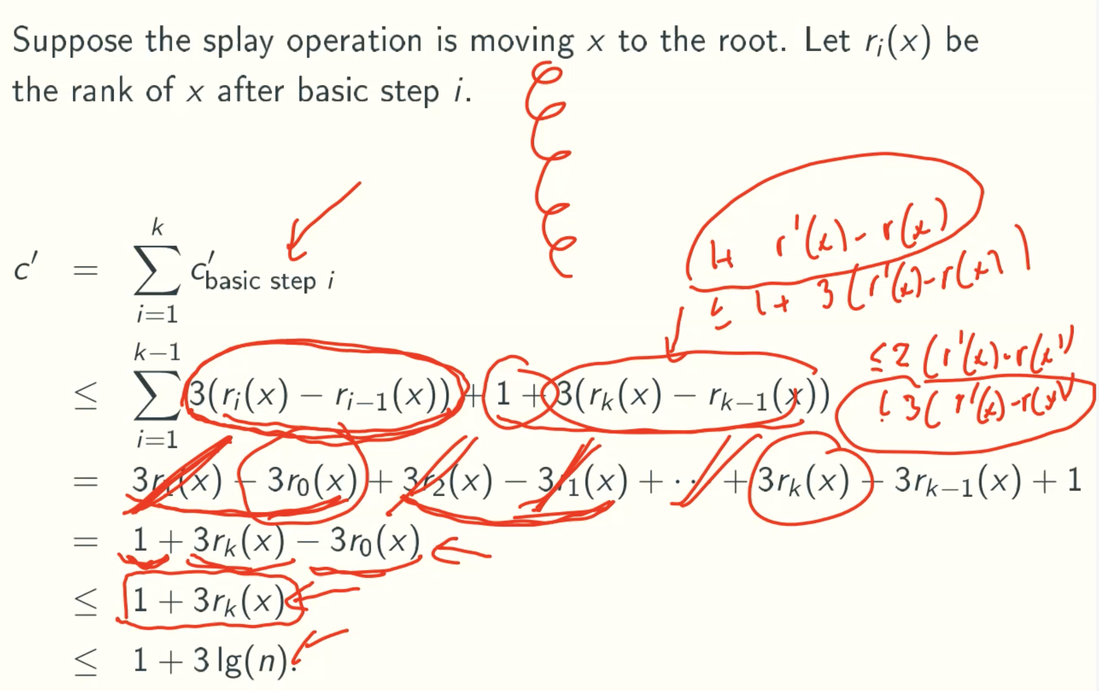
Amortized Analysis

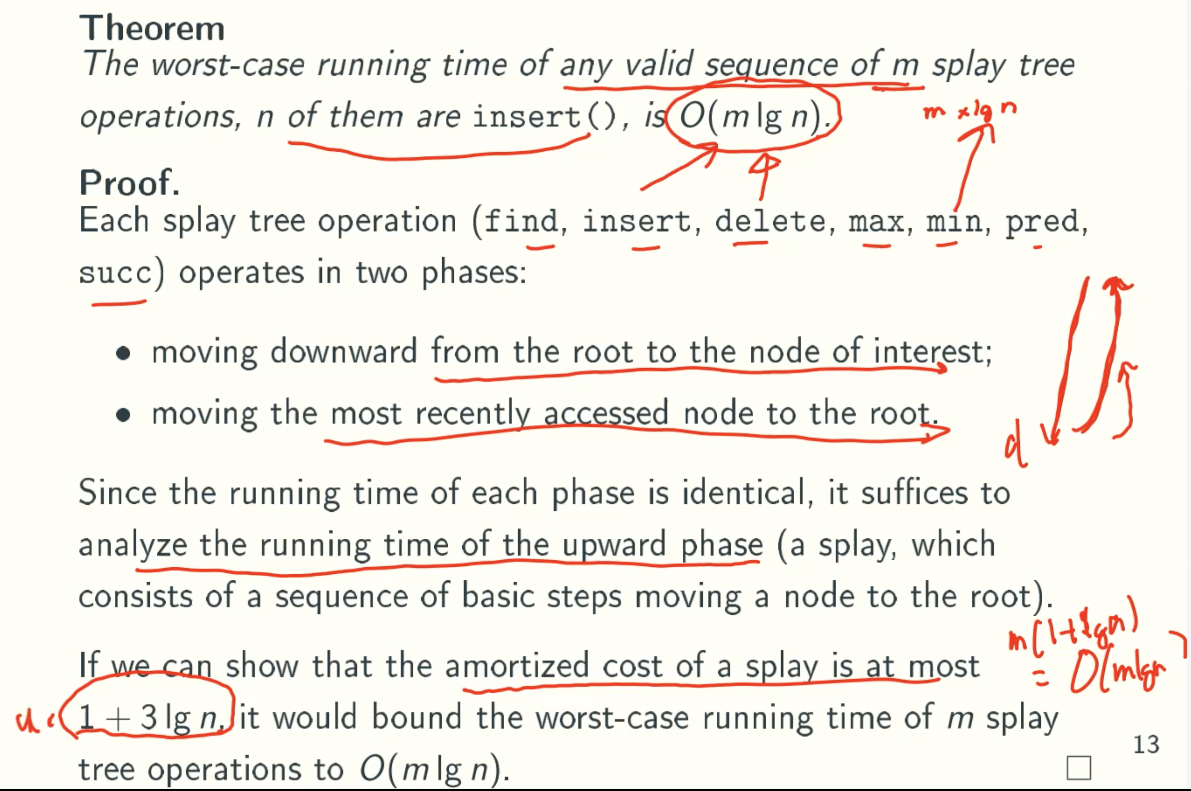
Amortized Cost Of A Splay Operation Is At Most 1 + 3lg(n)

Concave Functions

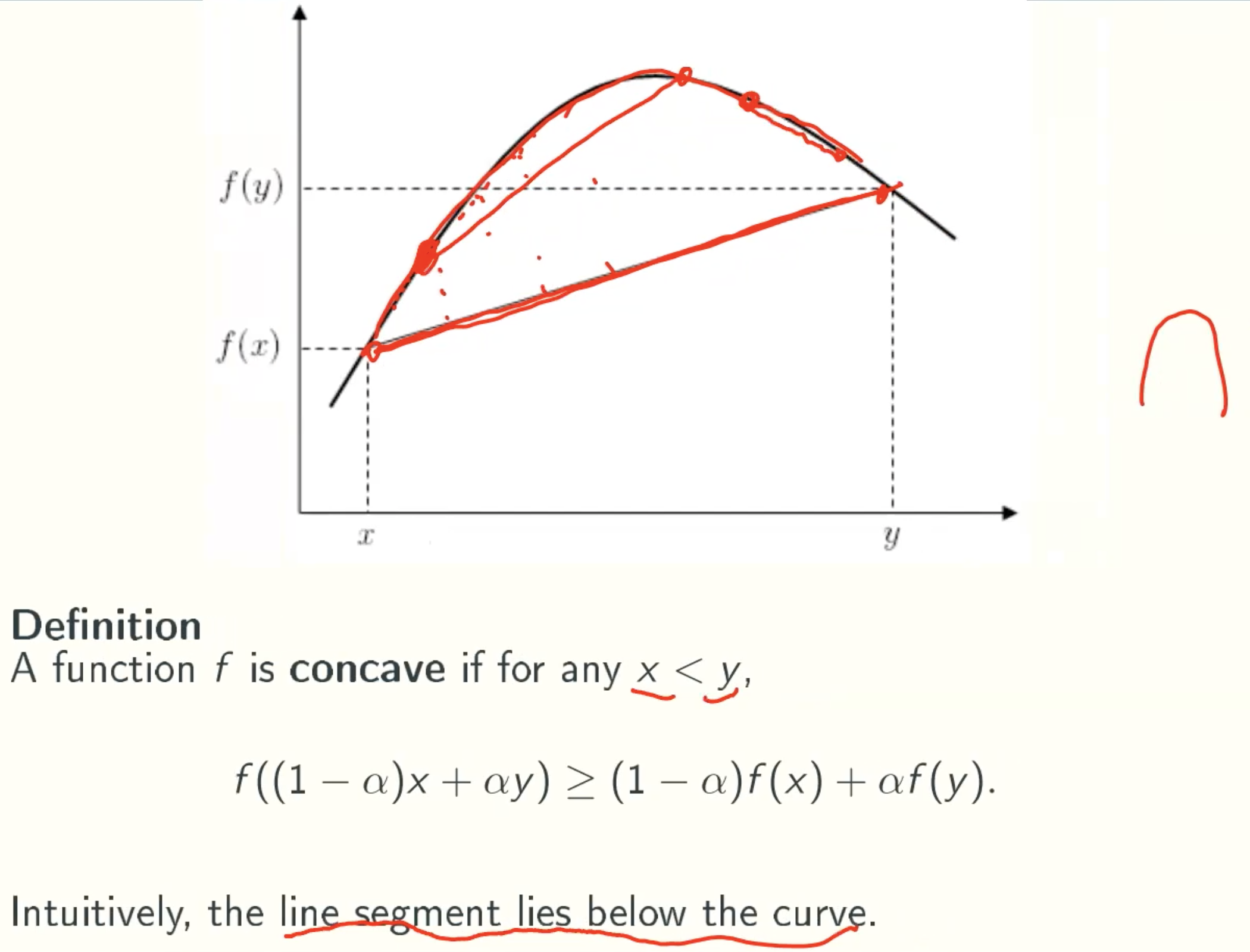
lg(x) + lg(y) ≤ 2lg((x+y)/2)

(lg(x)+lg(y))/2 ≤ lg((x+y)/2)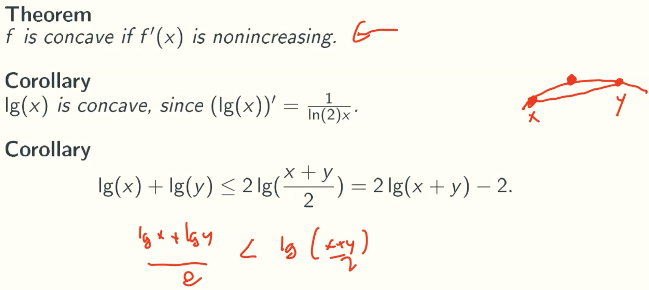

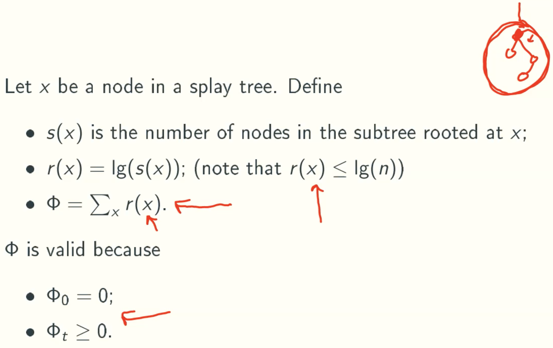
Potential Function

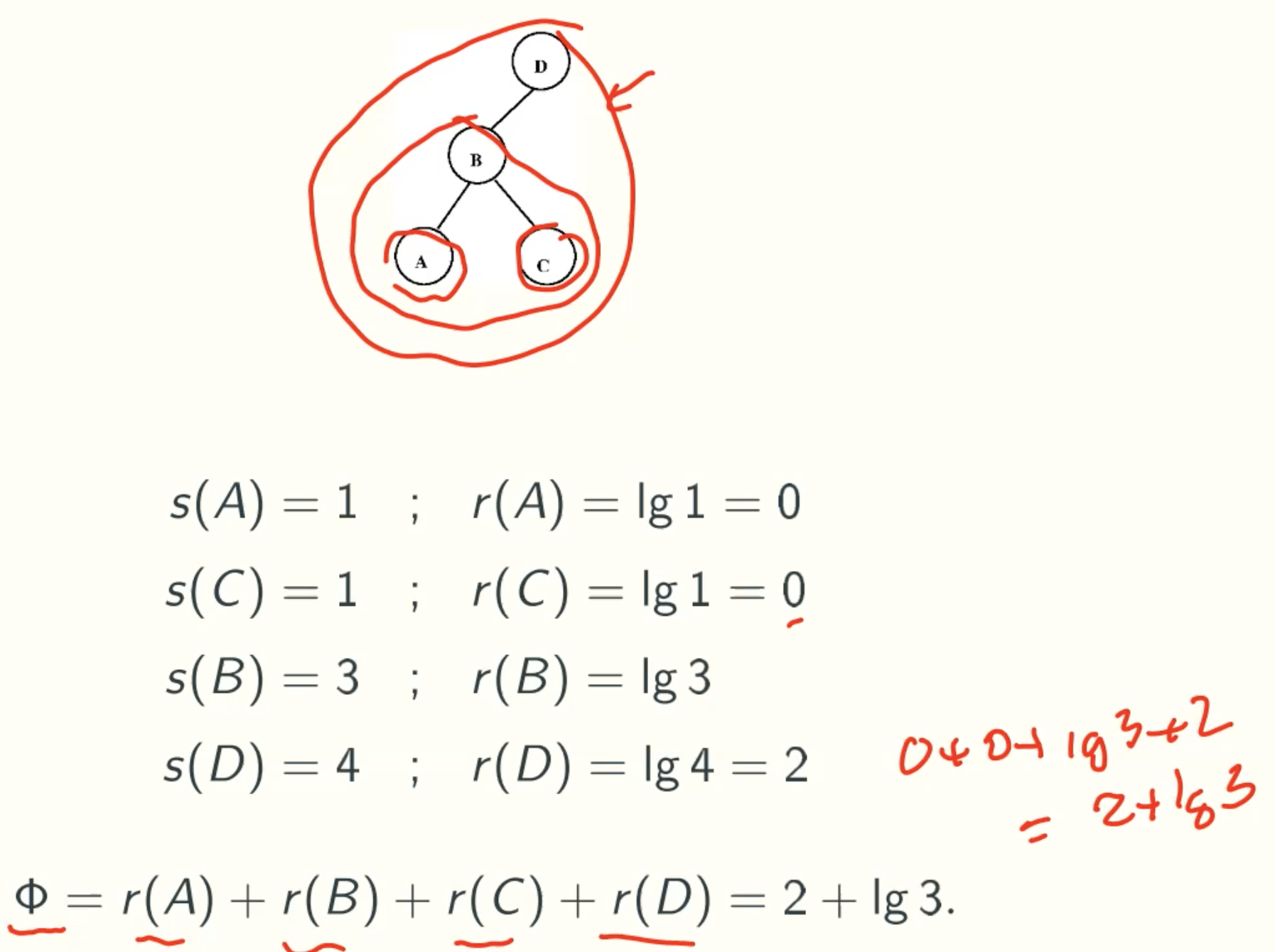
Example

Plan

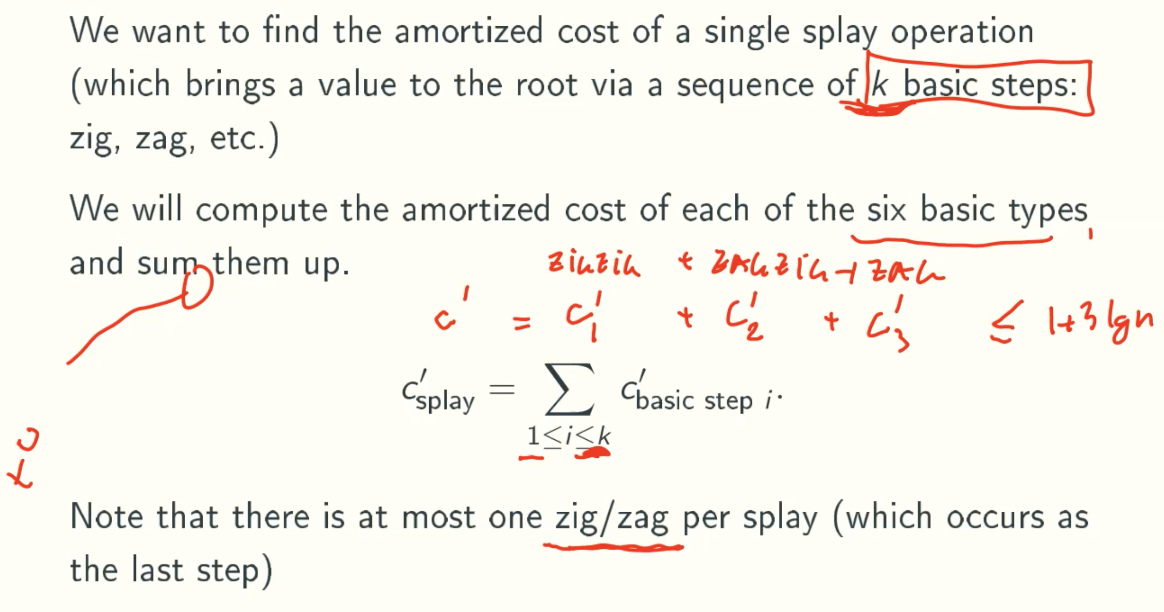
Notation

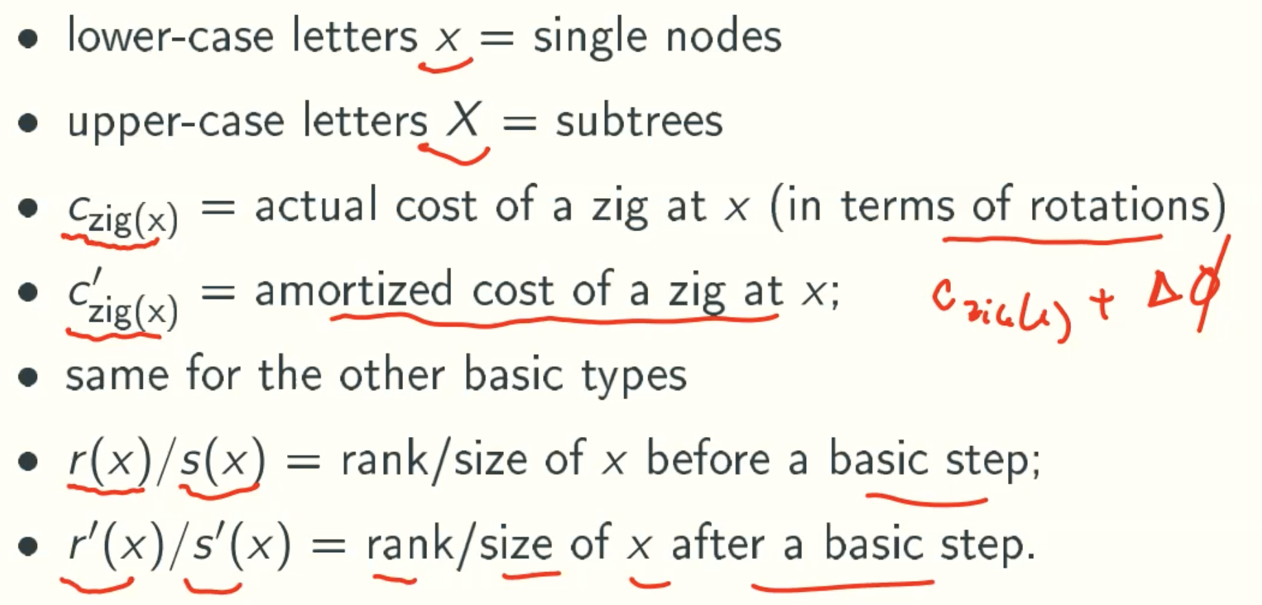
Zag and Zig

C’_zig(x) = C’_zag(x) ≤ 1 + r’(x) - r(x)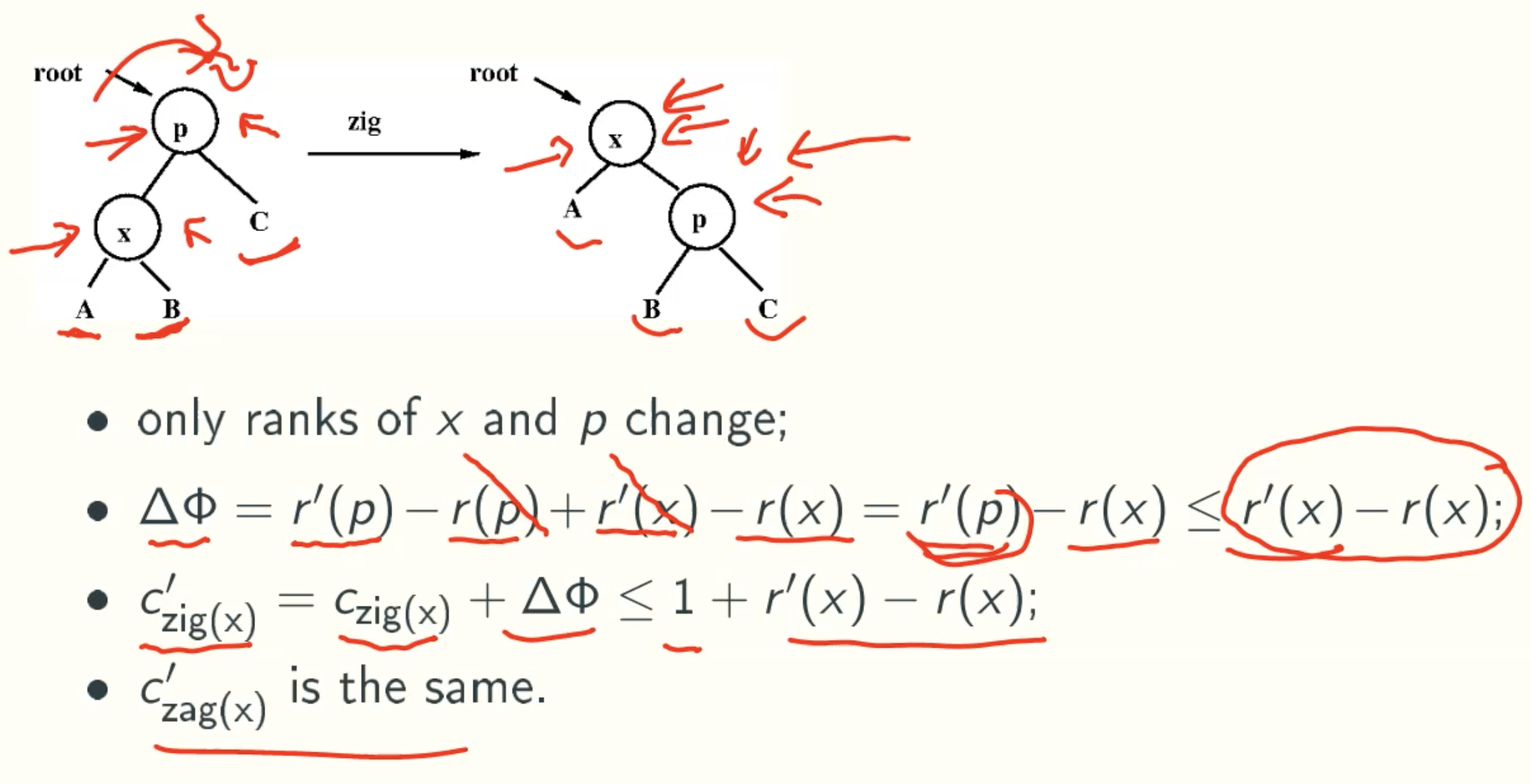

actual cost = rotation times

Zigzag and Zagzig

C’_zigzag(x) = C’_zagzig(x) ≤ 2(r’(x) - r(x))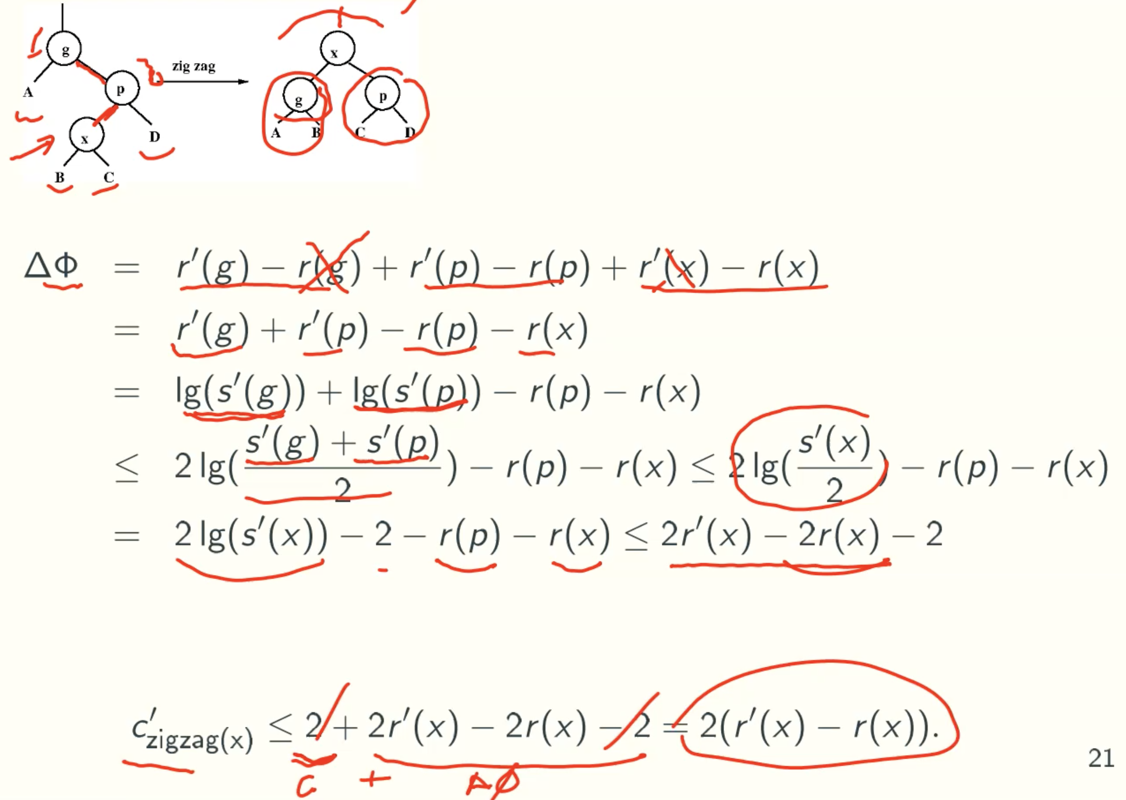

Zigzig and Zagzag

C’_zagzag(x) = C’_zigzig(x) ≤ 3(r’(x) - r(x))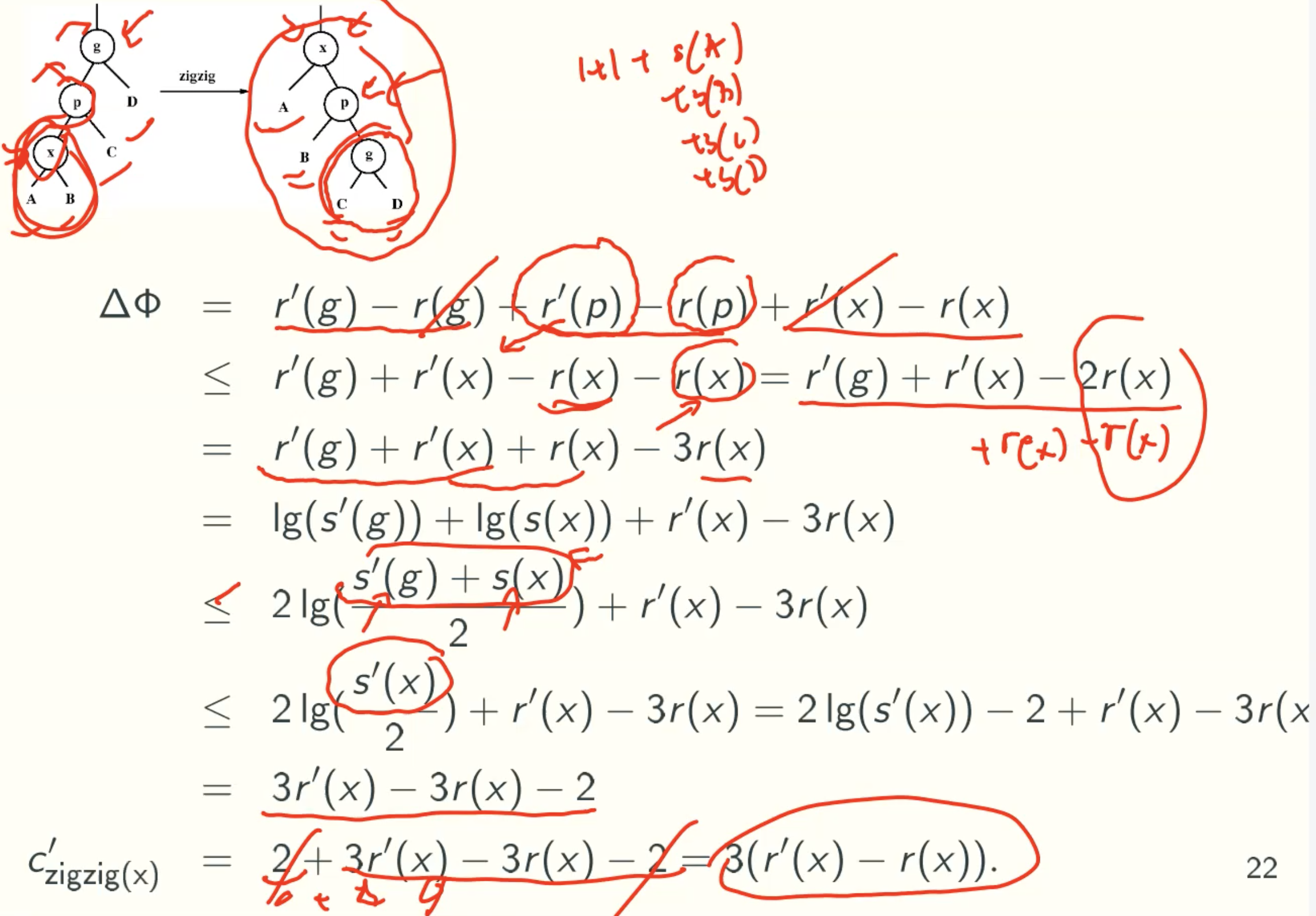

Total Amortized Cost

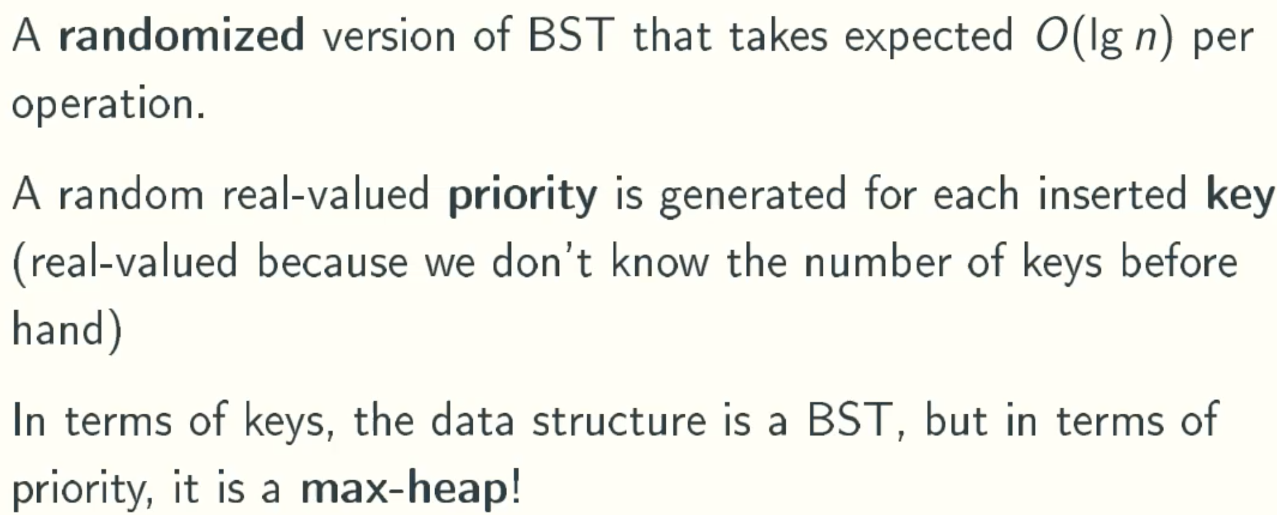
Treap

Overview

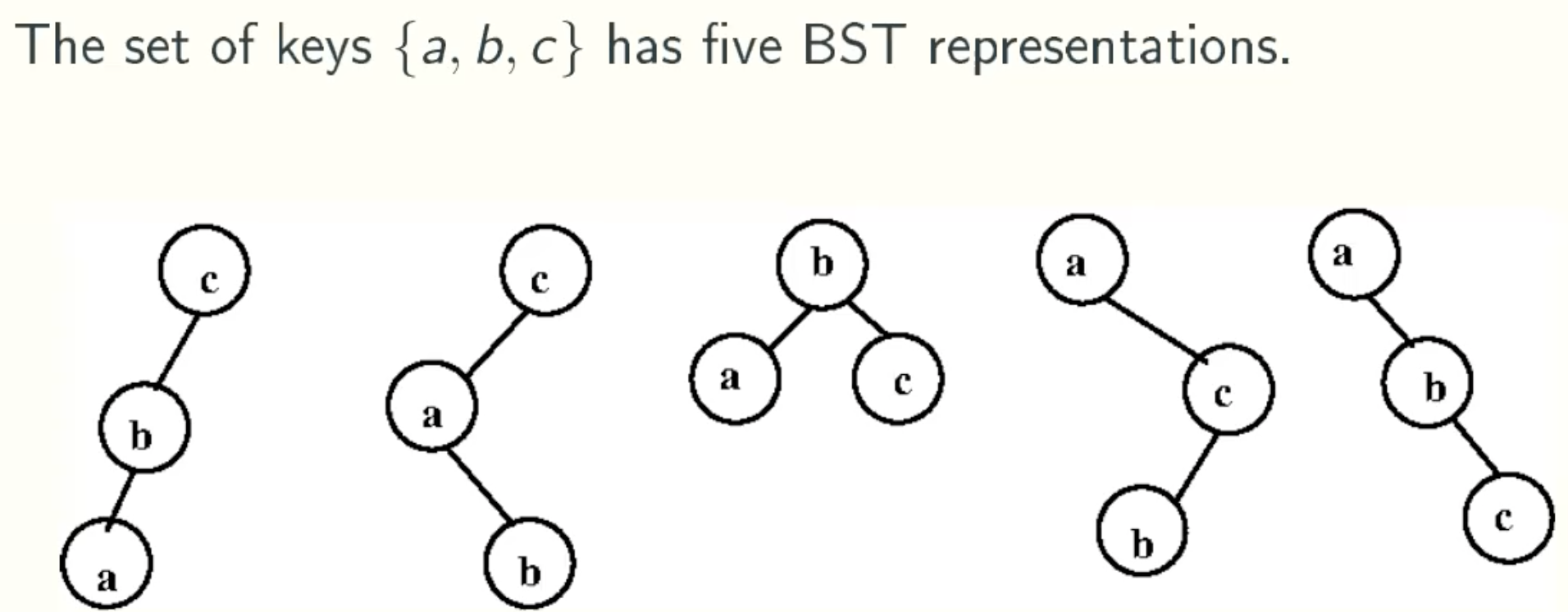
Treap Representations

Normal BST

Treap = BST + max-heap

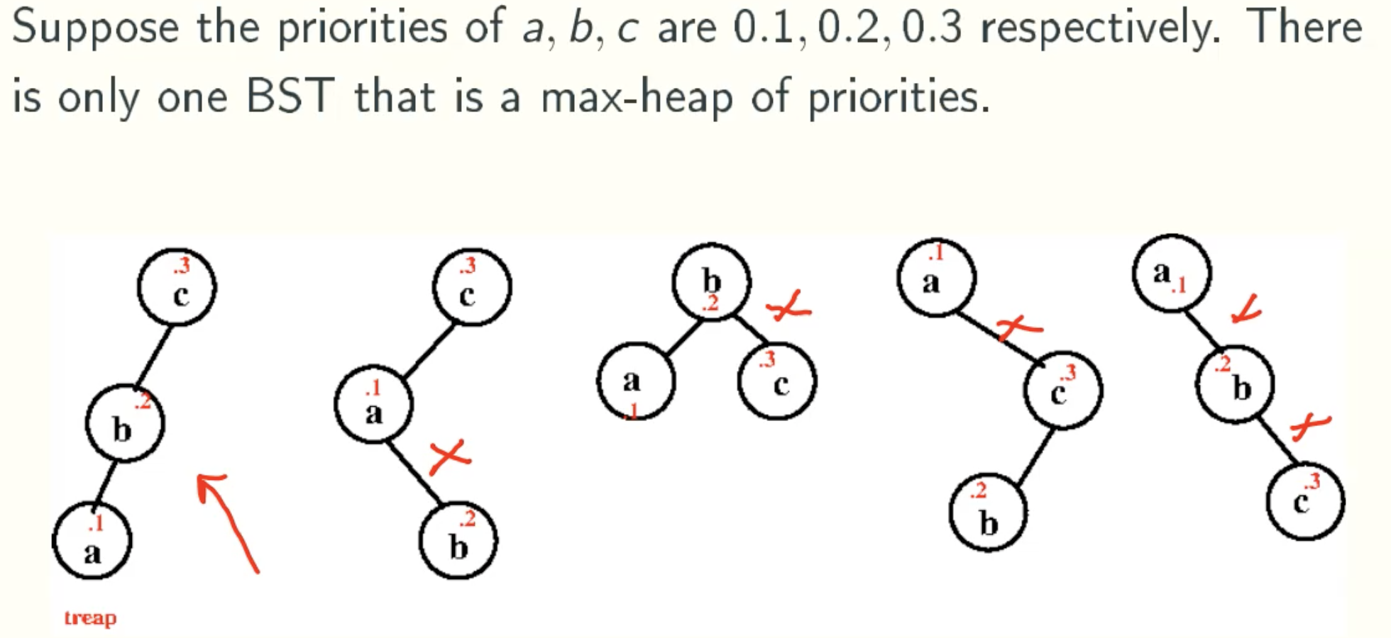
Unique Representation

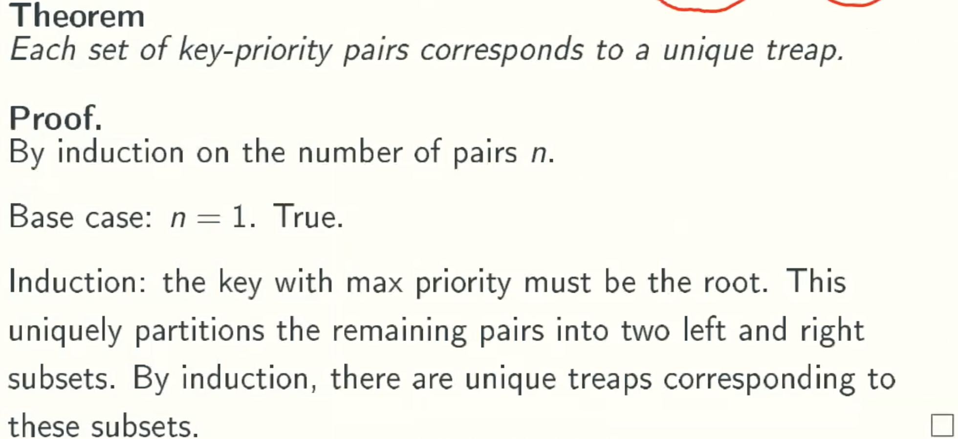
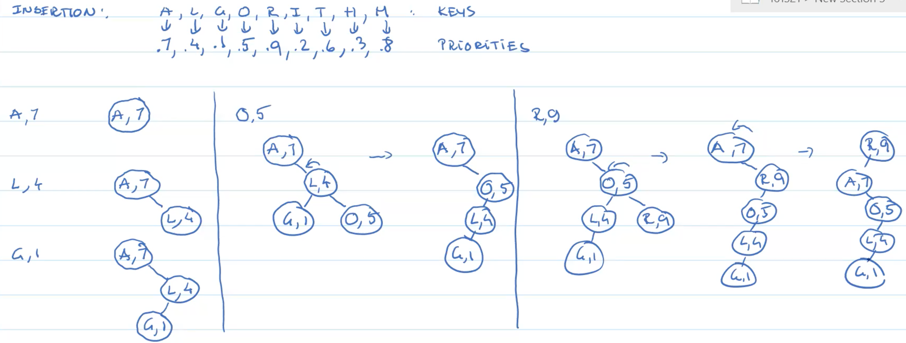
Treap Operation

1. max(), min(), pred(), succ(), find(): same for BST;
2. insert(): at a leaf as for BST, followed by a sequence of rotations up to restore heap order;
3. erase(): reverse of insert(), i,e.,a sequence of rotations down to a leaf while maintaining heap order(rotate the child wiht larget priority up), followed by removal.

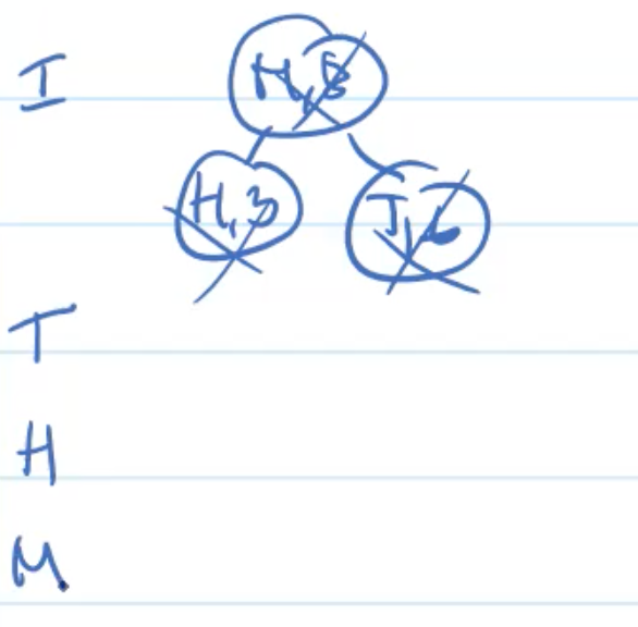
Example: Insertion

Example: Deletion

Analysis

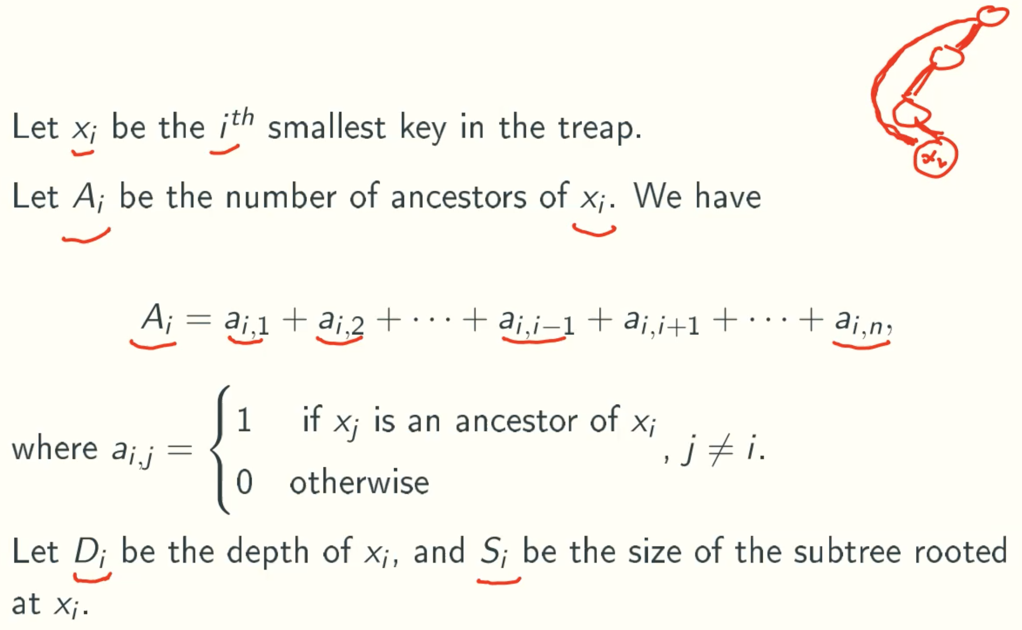
Notation

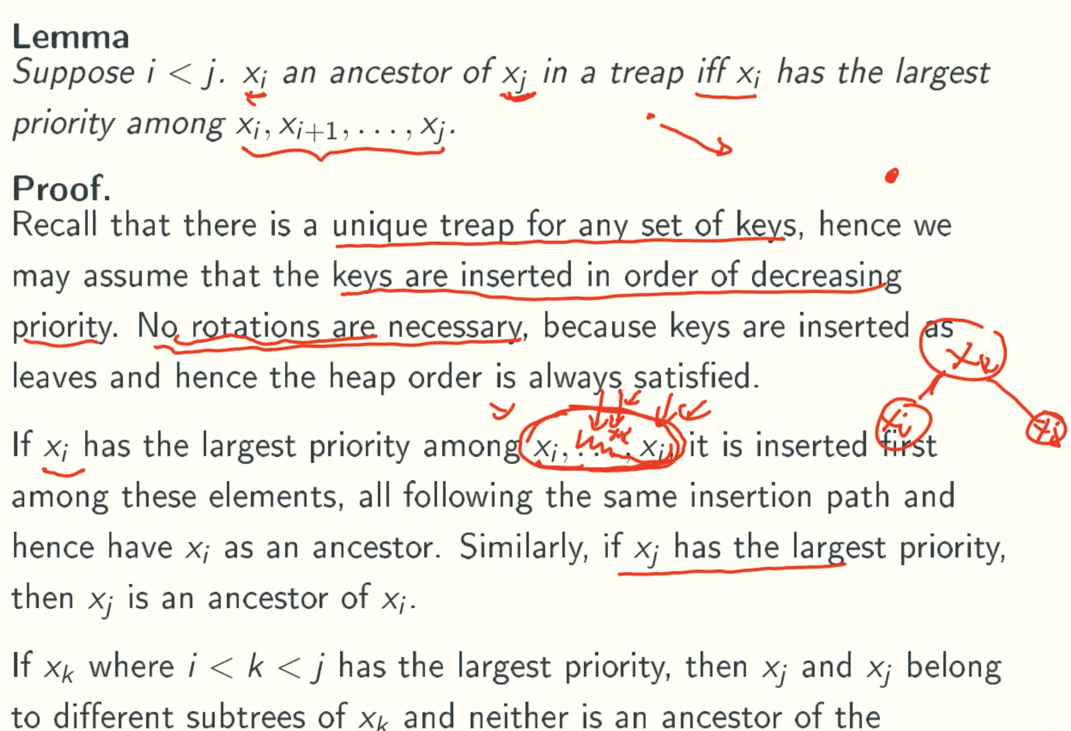
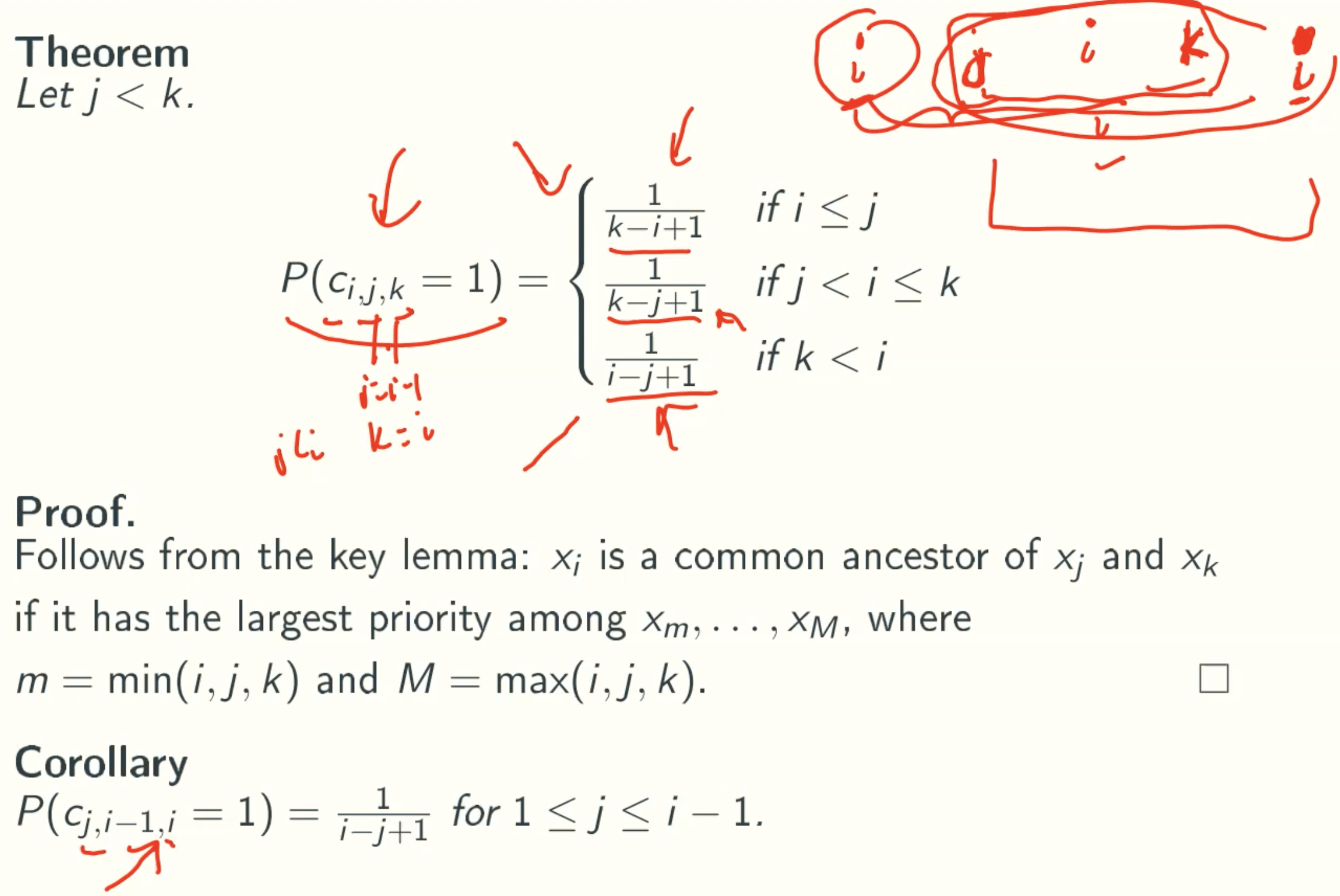
Key lemma

Expect Value

E[A_i]=⍬(lgn) 1≤i≤n

Expect depth and size

Left And Right Spine

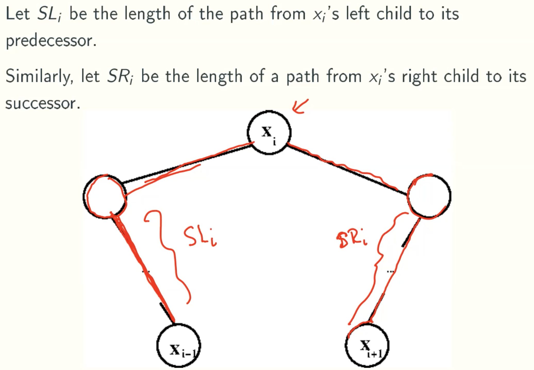
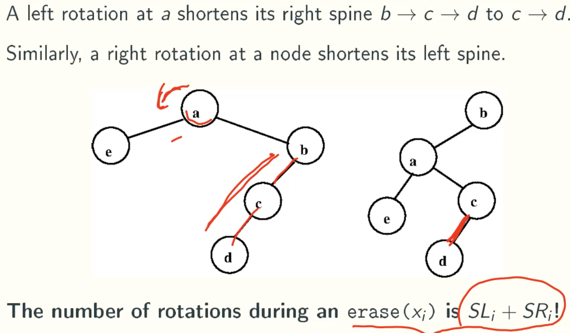
Left Rotation Shortens Right Spine

Expect Length Of Left Spine Of X_i

P(C_i,j,k = 1)

E[SL_i] = 1 - 1/i

Same with E[SL_i], E[SR_i] = 1 - 1 /(n+1-i)

Expection Running Time Of Treap Operations

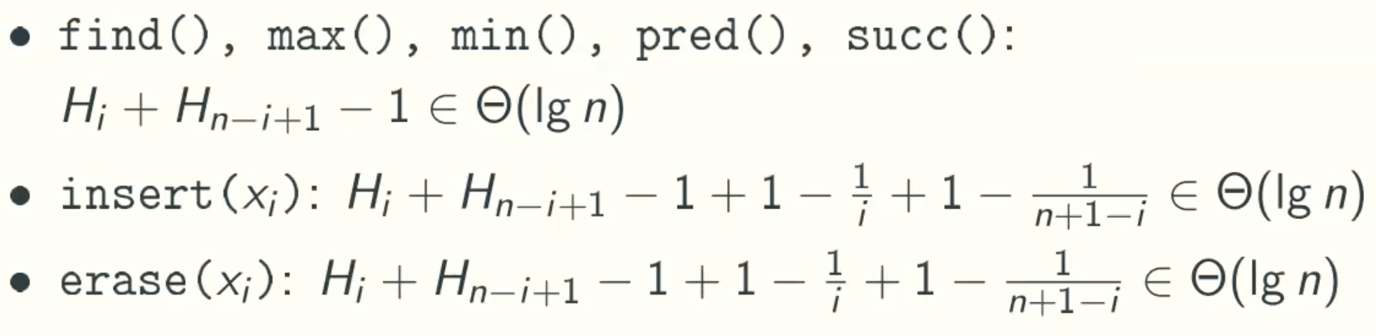
The Rotation in insertion and erase is at most O(2)

Skip List

Overview

Motivation

Worst-Analysis

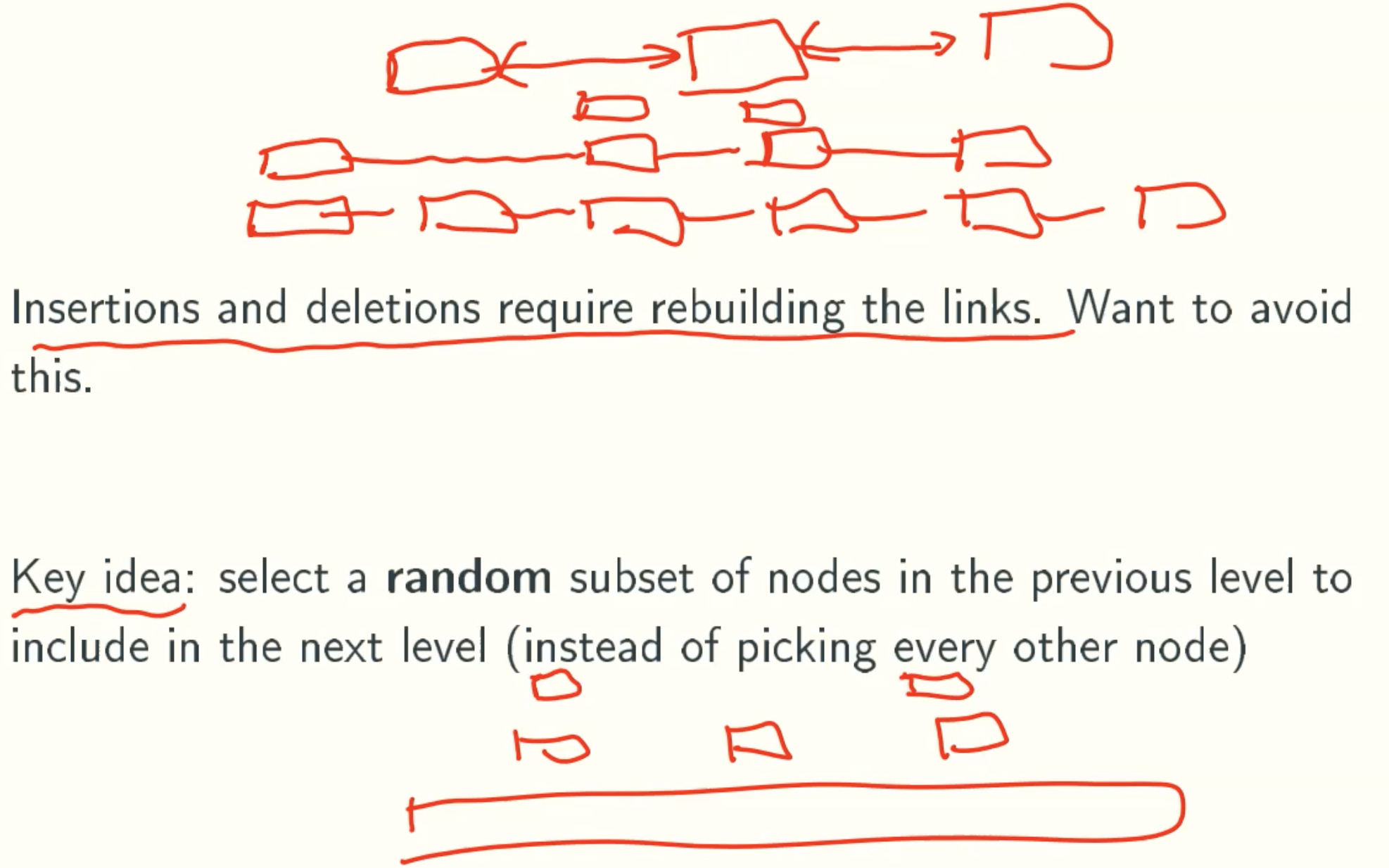
Insertion&Deletion

Skip List Operations

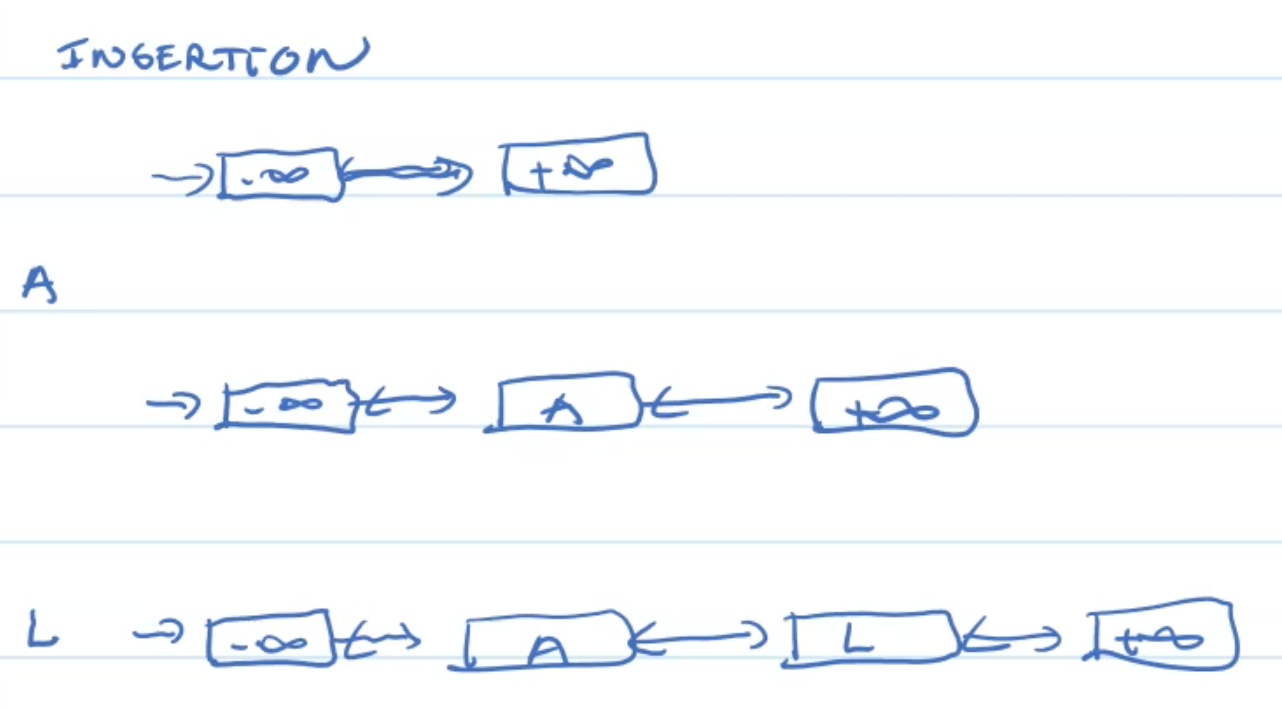
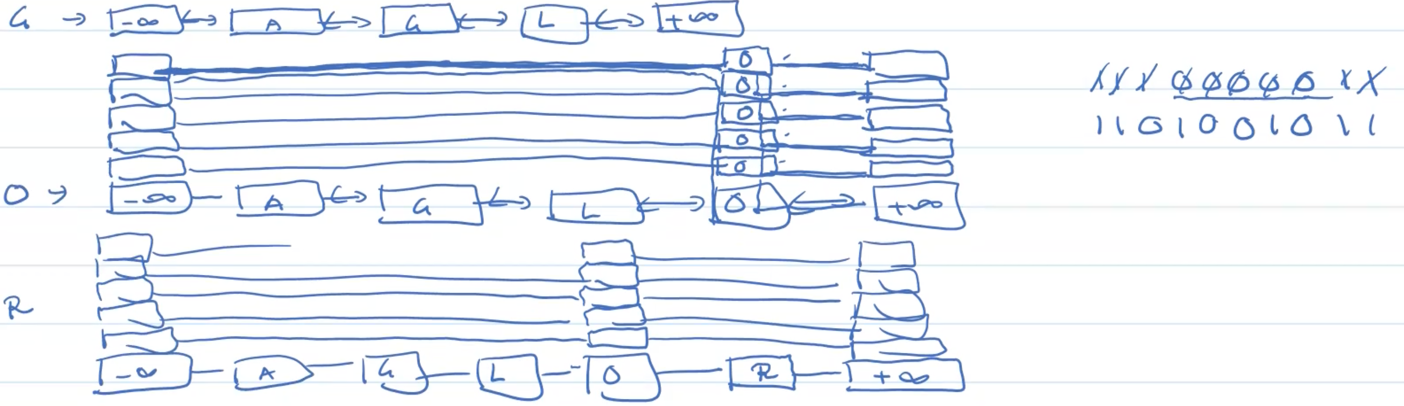
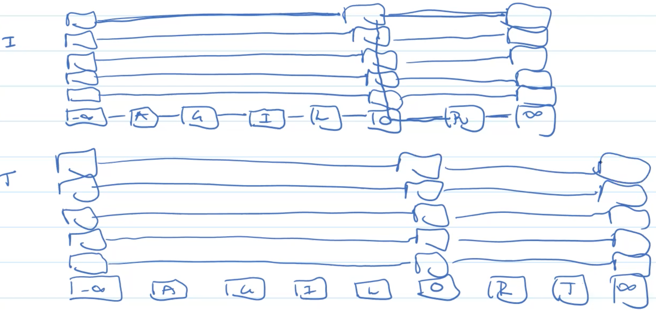
Example: Insertion

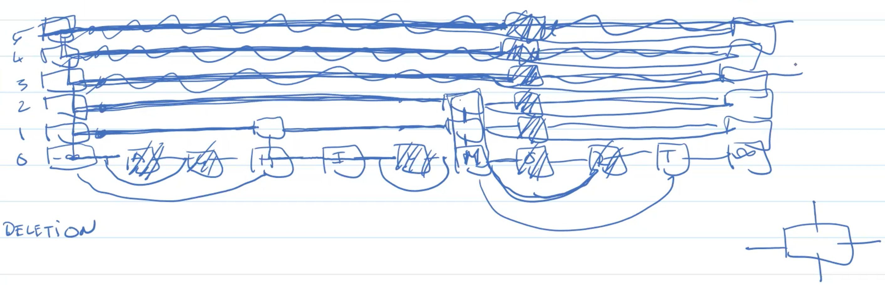
Example: Deletion

Analysis

Notation

• S: size of skip lists for a given set of n keys
• S_i: size of level-i list(bottom list is at level 0)
• H: number of levels
• T_op: number of comparisons by operation op()

Expection Of S_i

Expection Of S

Expection Of H

∑ n/2ⁱ = ∑ n * 1/2^lgn * 1/2ⁱ = ∑1/2ⁱ = 1

Expection of T_op

A find need a horizontal move only when the before nodes toss head. Head means they will build tower.

Minimum-Weight Spanning Trees

Definition

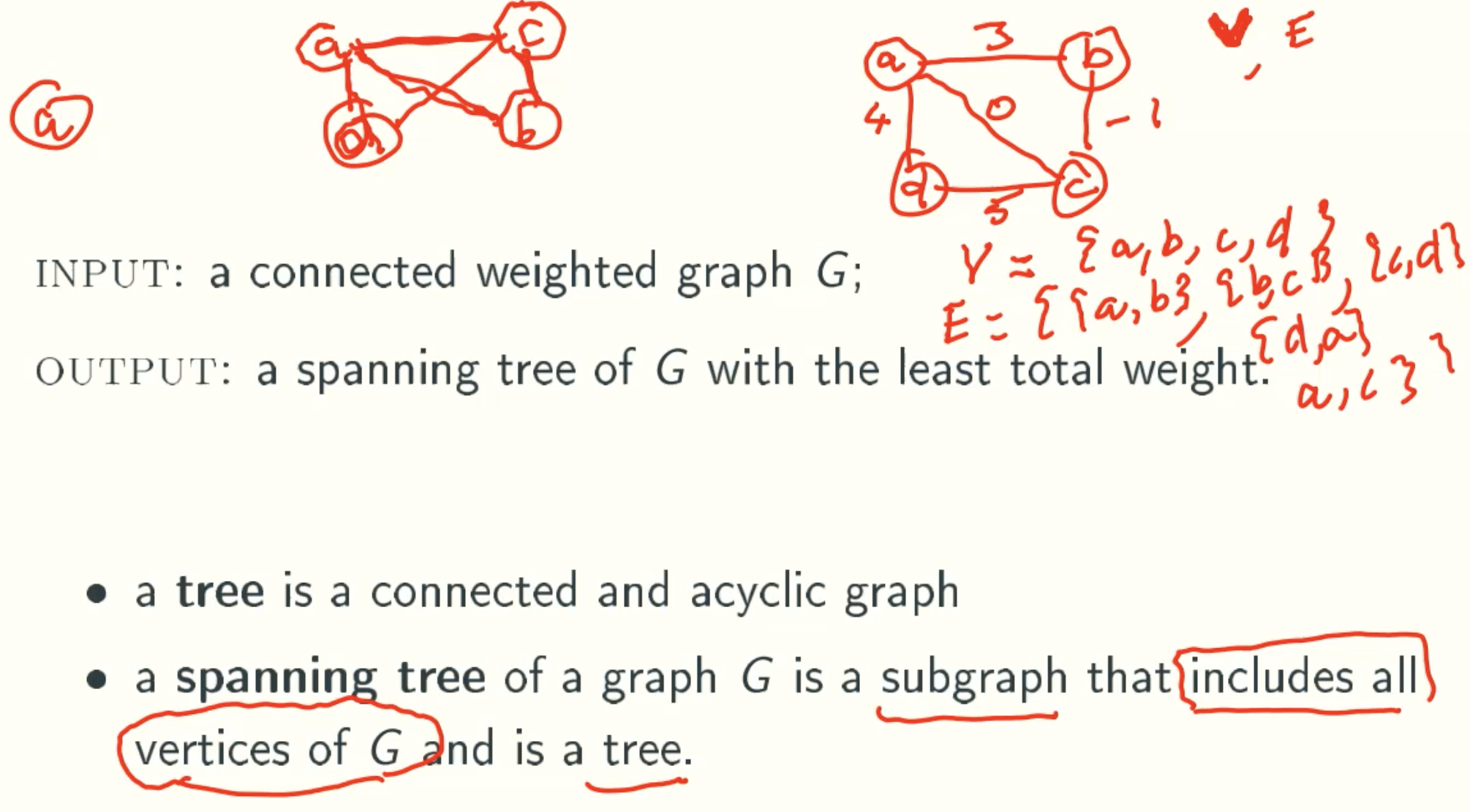
Example

Facts

• G has a spanning tree iff it is connected
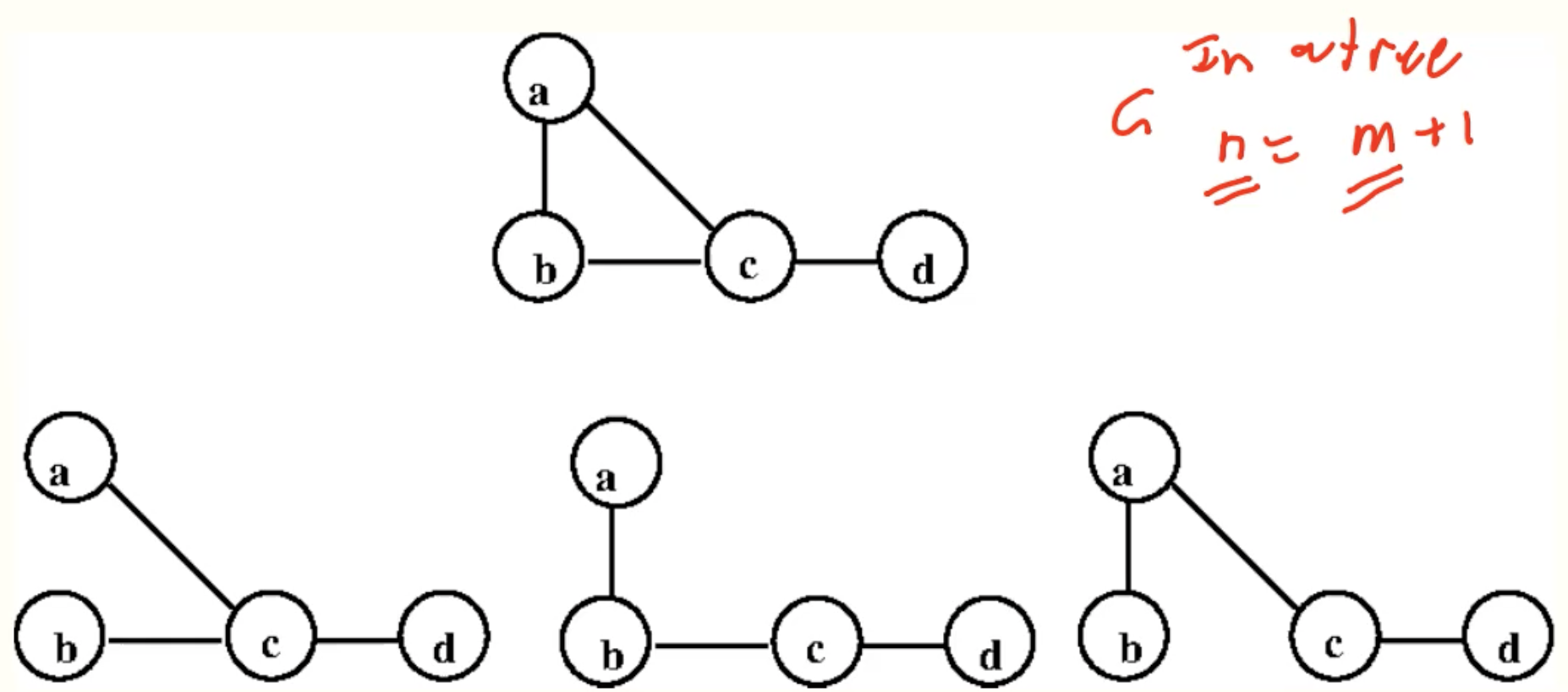
• Let T be a graph with n vertices and m edges. The following are equivalent
  • T is a tree
  • T is connected and n = m + 1
  • T is acyclic and n = m + 1
  • there is a unique path between any two vertices in T.
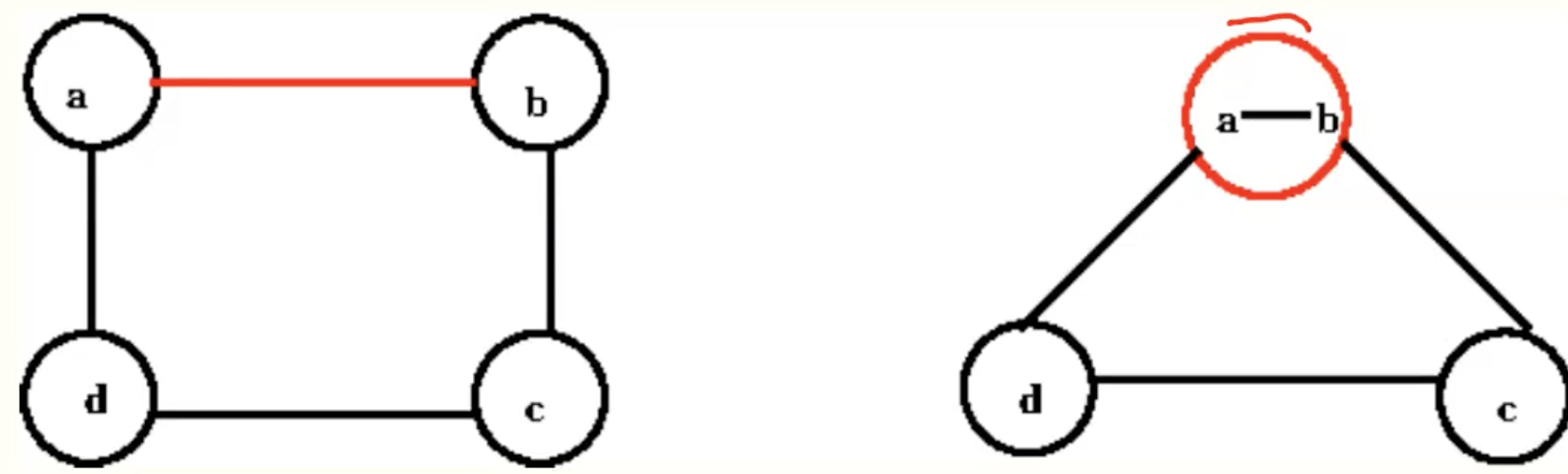
• adding an edge between two existing vertices of a tree creates a cycle; removing an edge from this cycle yields back a tree.

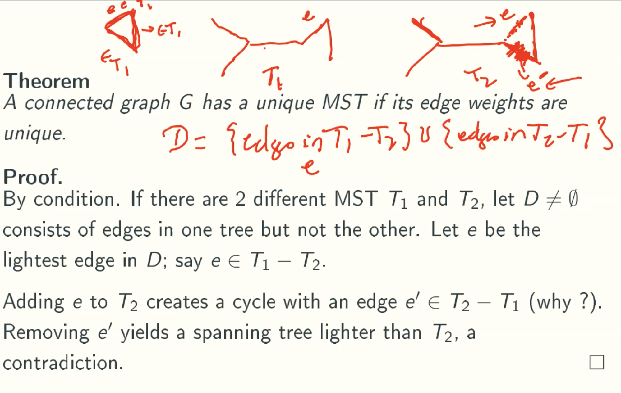
Theorem: Unique weights means unique MST

Converse: Unique MST doesn’t means unique weights

That is beacuse if n = m + 1, we just has one subgraph.

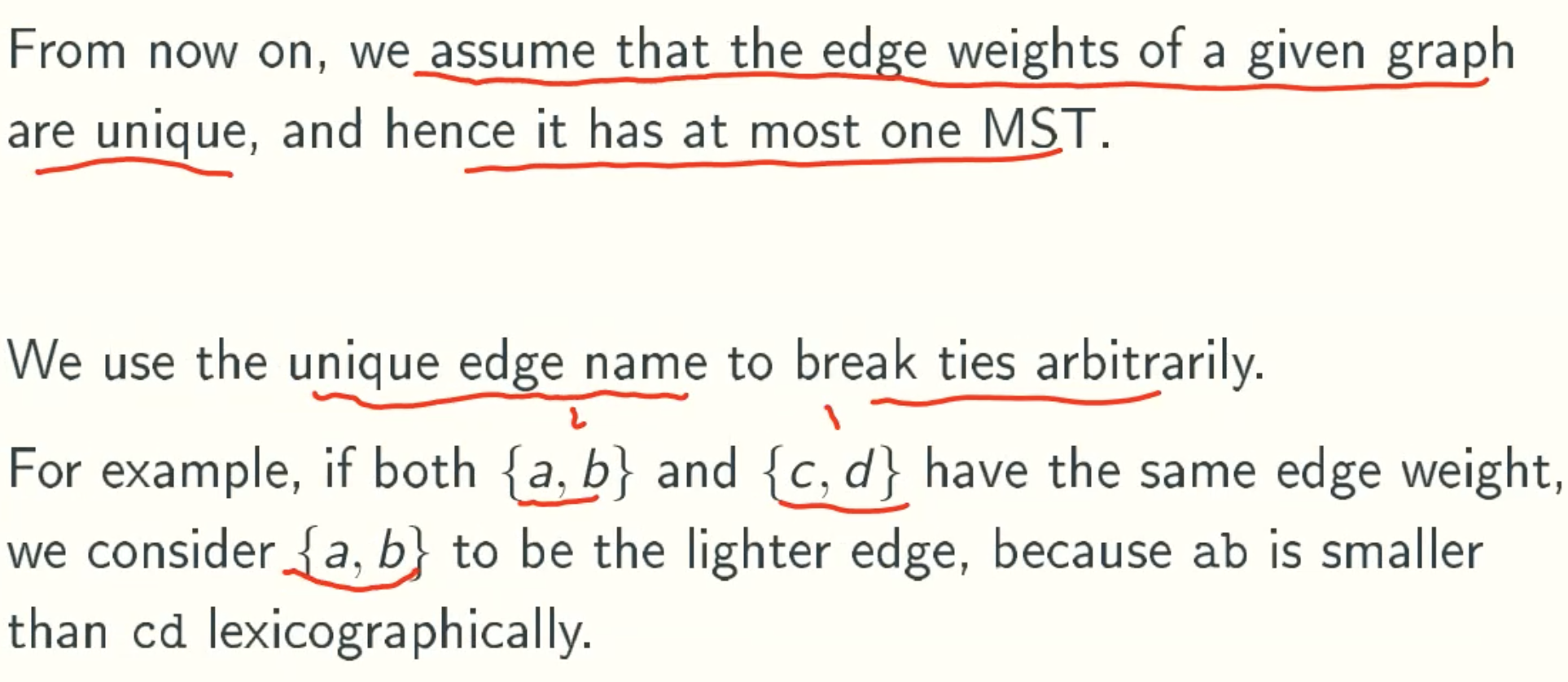
Key assumption

MST Algorithms: Kruskal, Prim, Boruvka

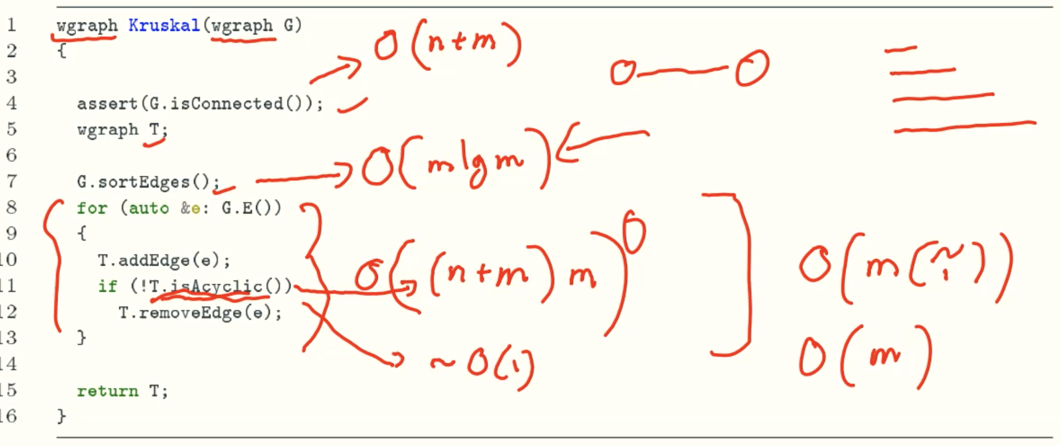
Kruskal’s algorithm

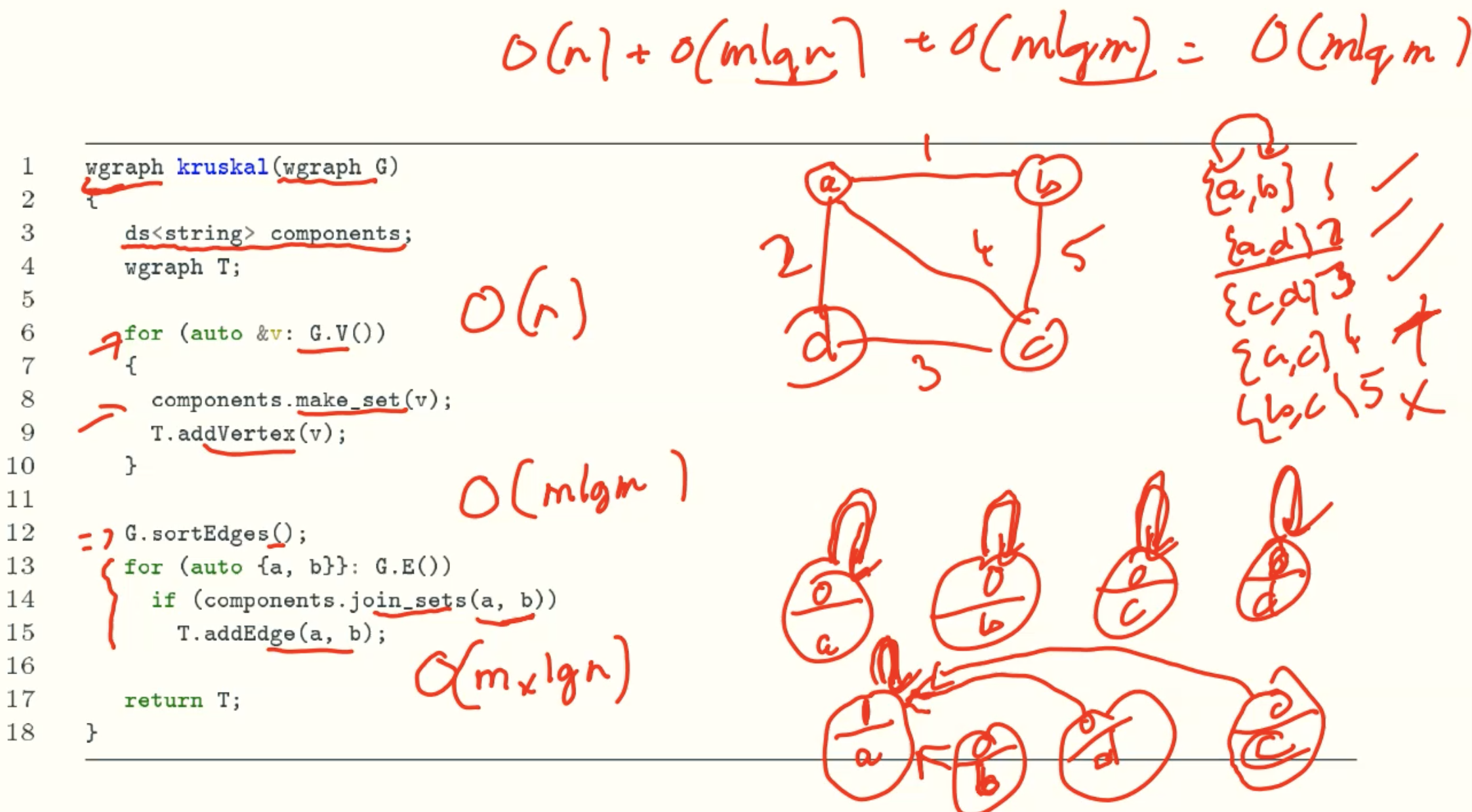
Code

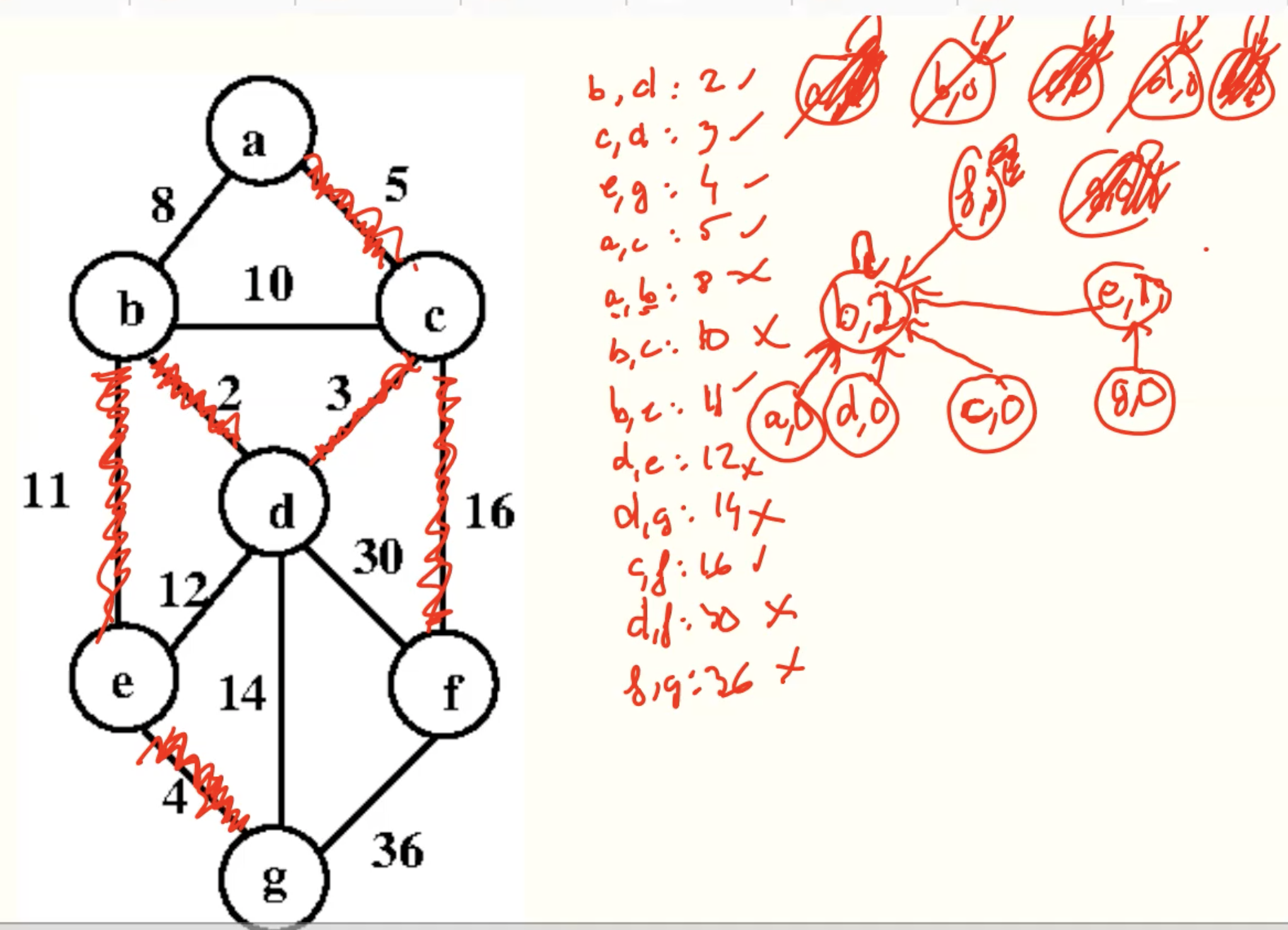
Example

Analysis

• Naive implementation using BFS/DFS: O(m(n+m))
• Using disjoint sets: O(mlgn)

Edge Contraction

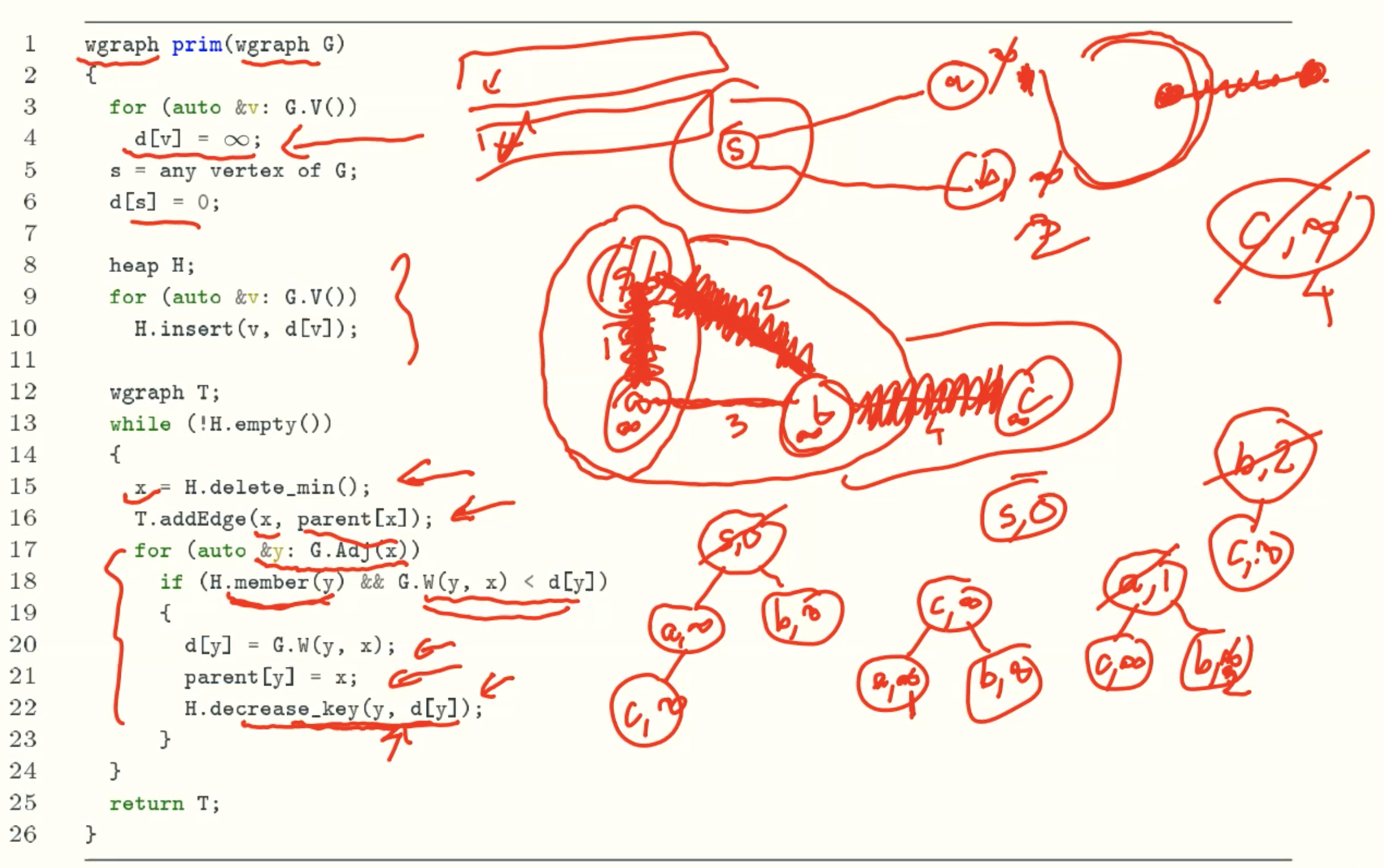
Prim’s algorithm

Code

Example

Analysis

• Navie implementation using edge contraction is expensive
• Implementation using a min-heap takes O(mlgn) time
• Implementation using a Fibonacci heap takes O(m + nlgn) time

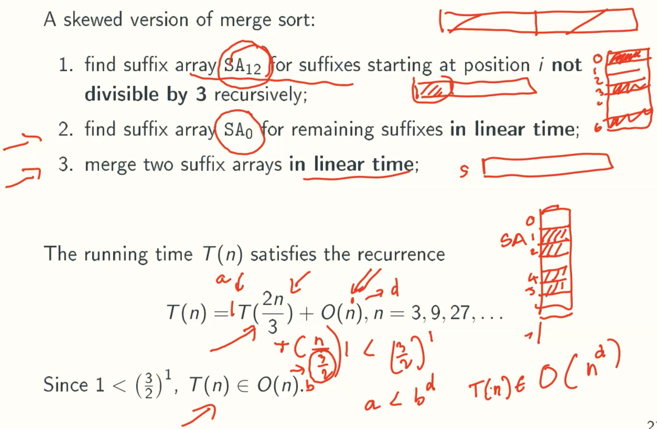
__Note Why O(m + nlgn) < O(mlgn)__
Here m is the vertexes, n is the edges
since n² ≥ m ≥ n-1, in worst-case every node is connected, so m = n² in that case, O(n² + nlgn) < O(n²lgn)

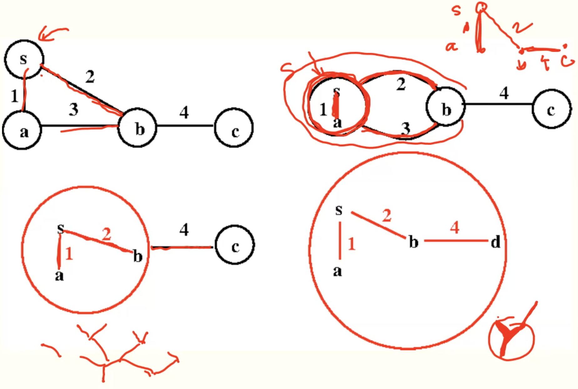
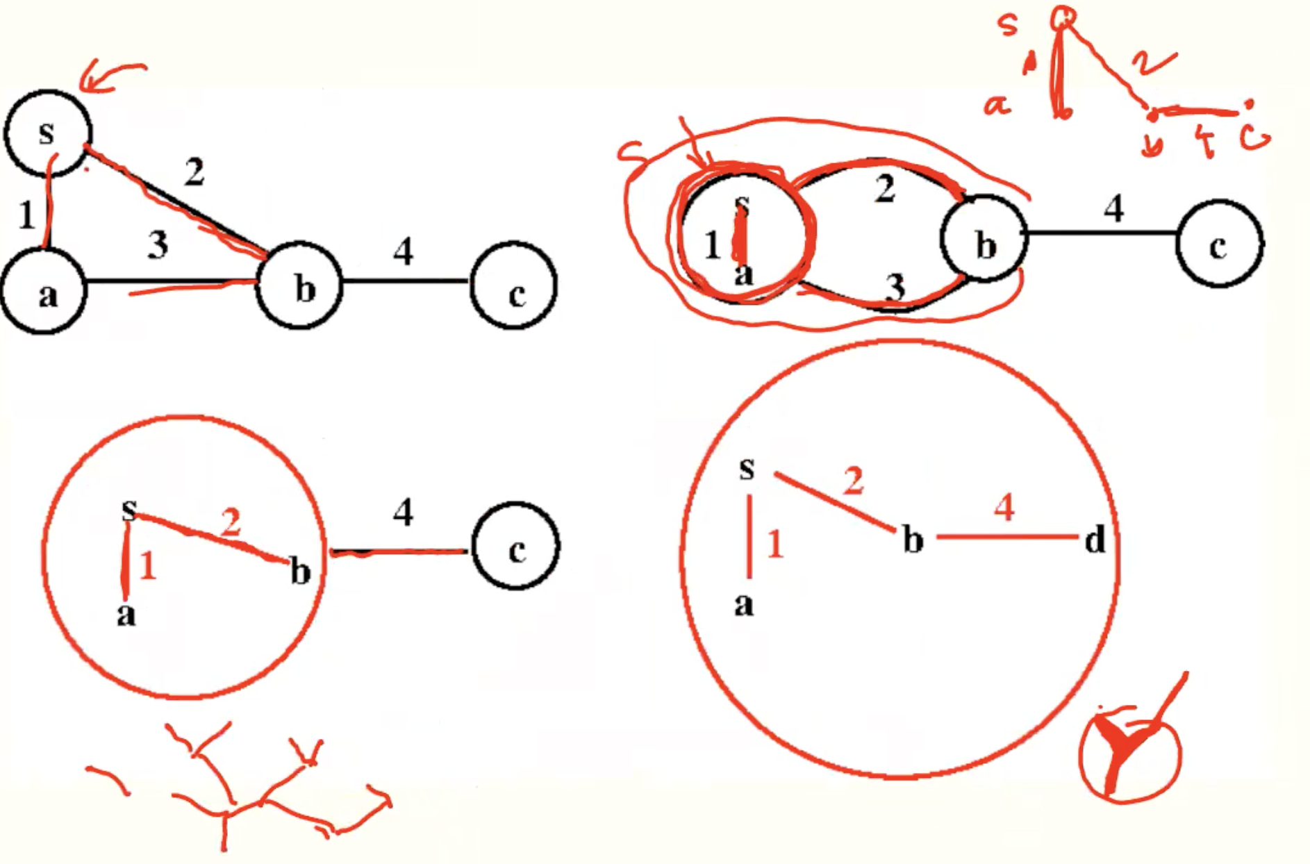
Boruvka’s algorithm

Code

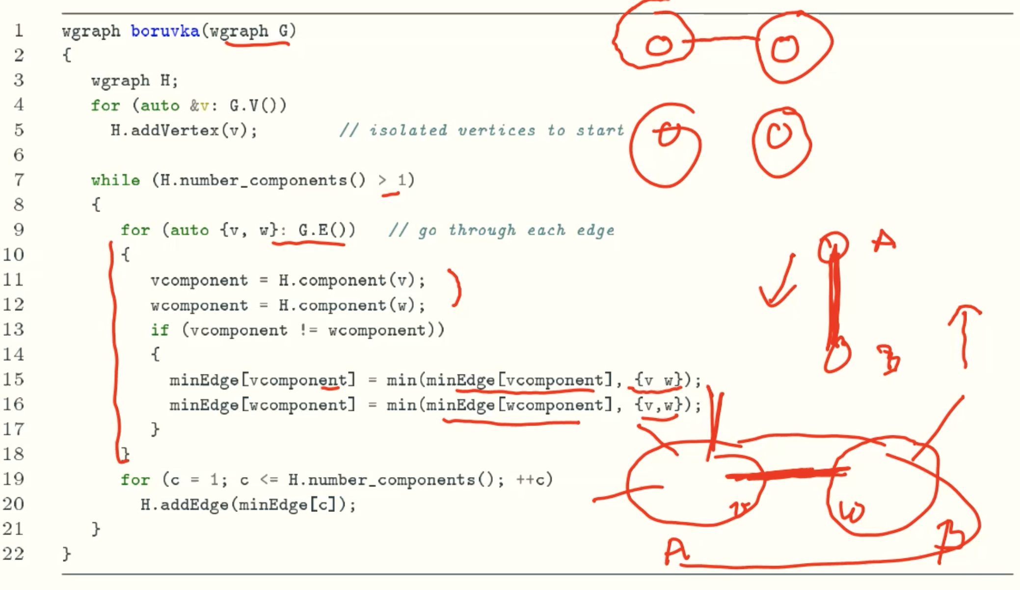
Example

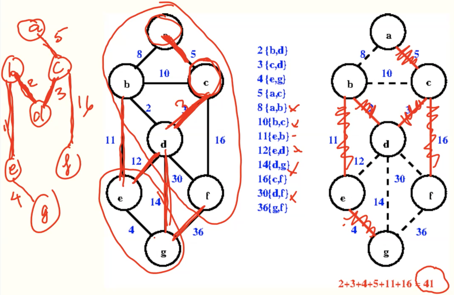
Analysis

• takes O(lgn) rounds, since the number of components is at least halved each round.

Disjoint Sets

Overview

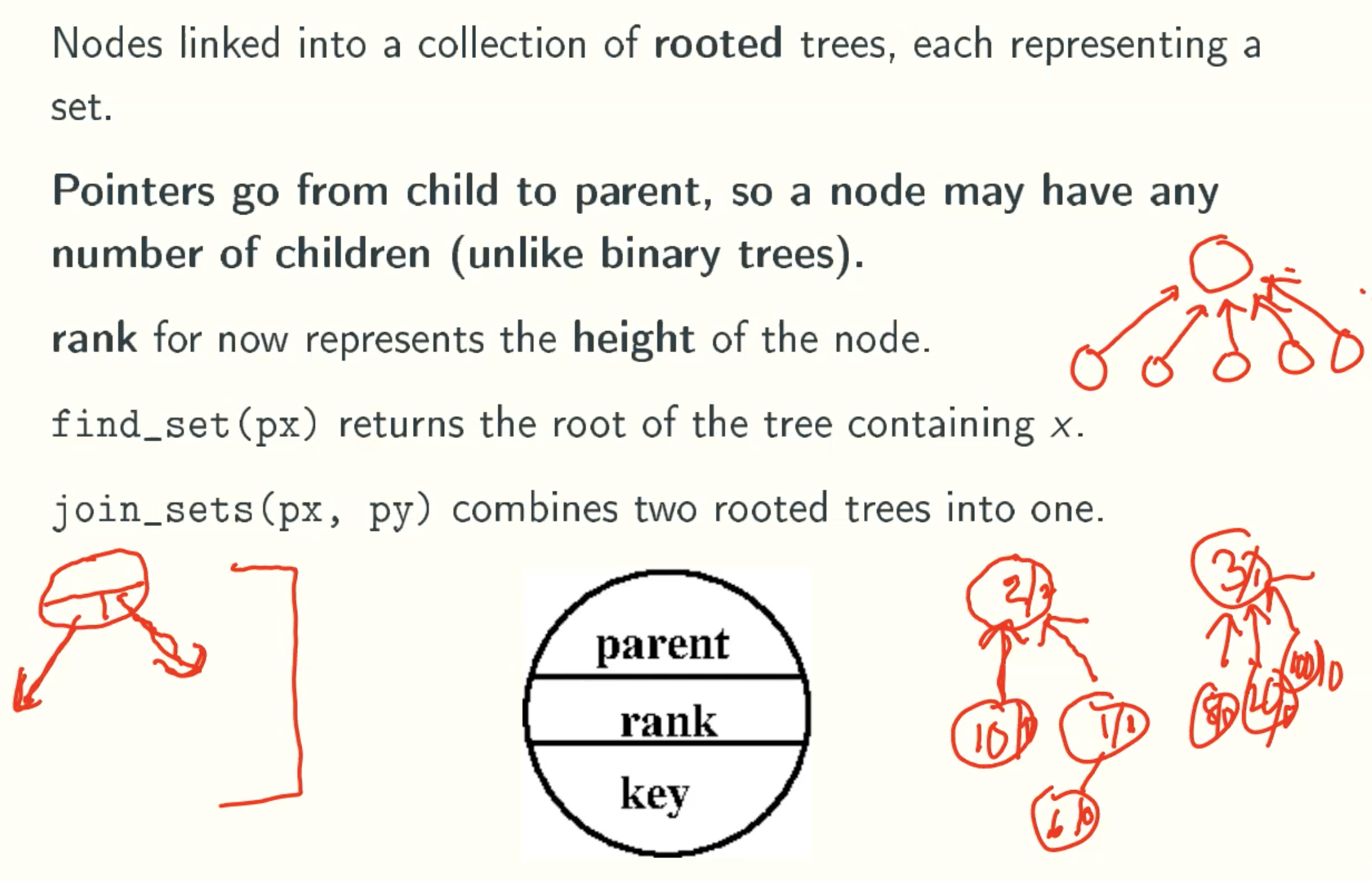
A data structure to maintain a collection of sets of objects, Supported operations are:

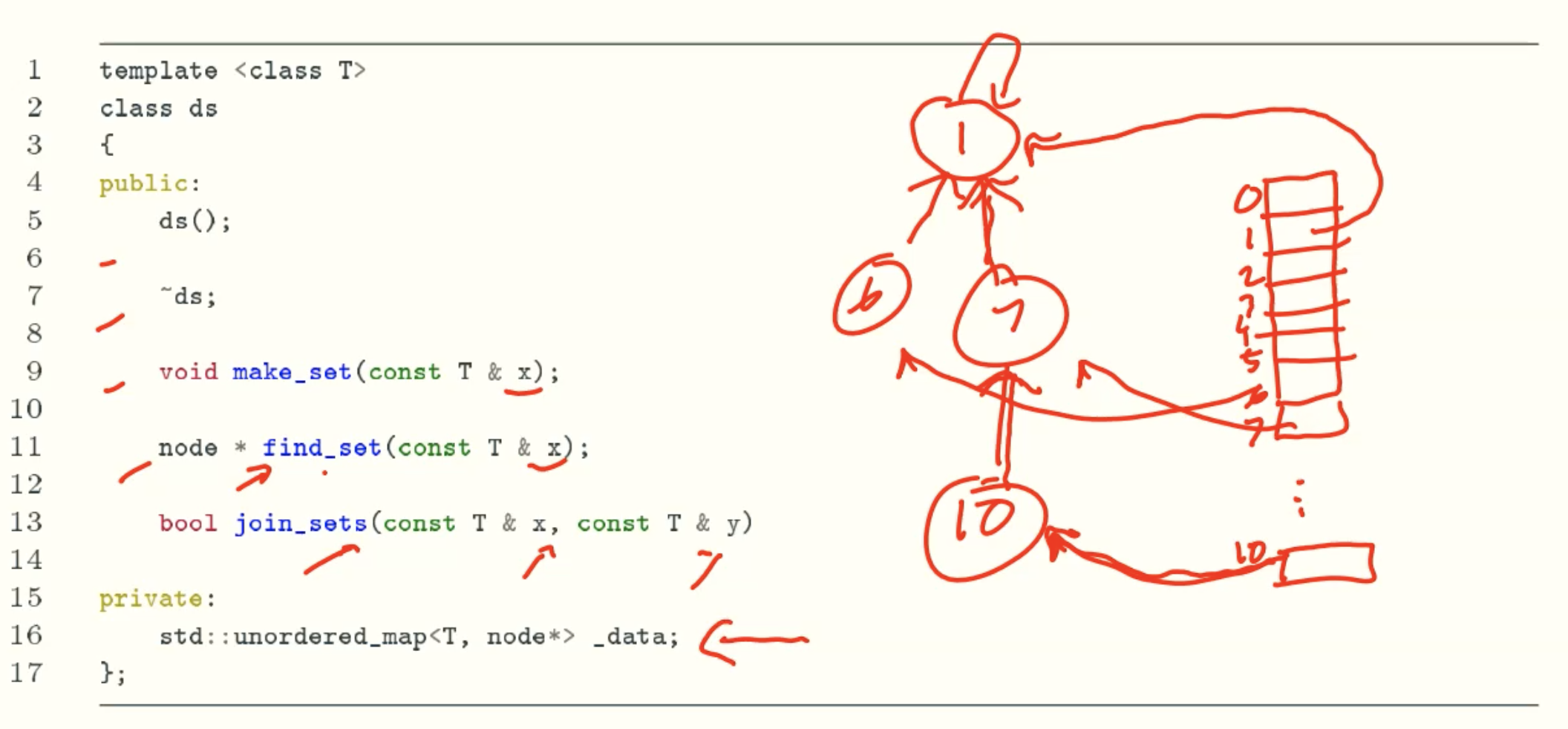
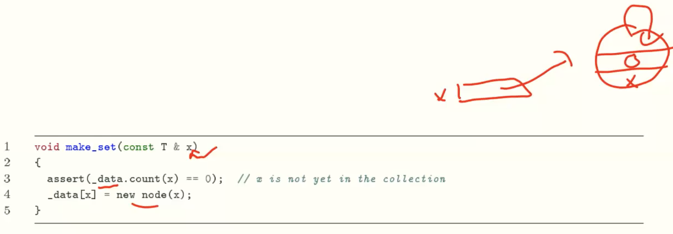
• make_set(x): create a new set with one element x;
• find_set(px): returns the set containing x, given its pointer;
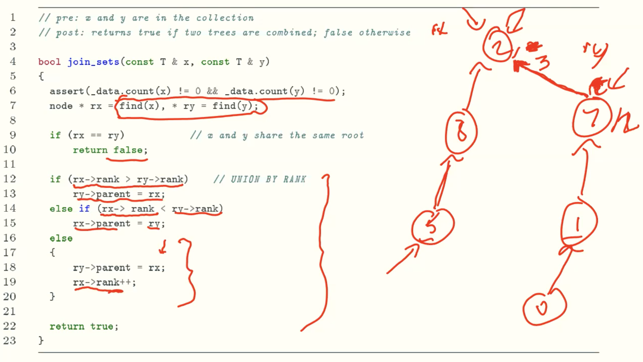
• join_sets(px, py): combine the sets containing x and y, given their pointers.

Representation

Implementation

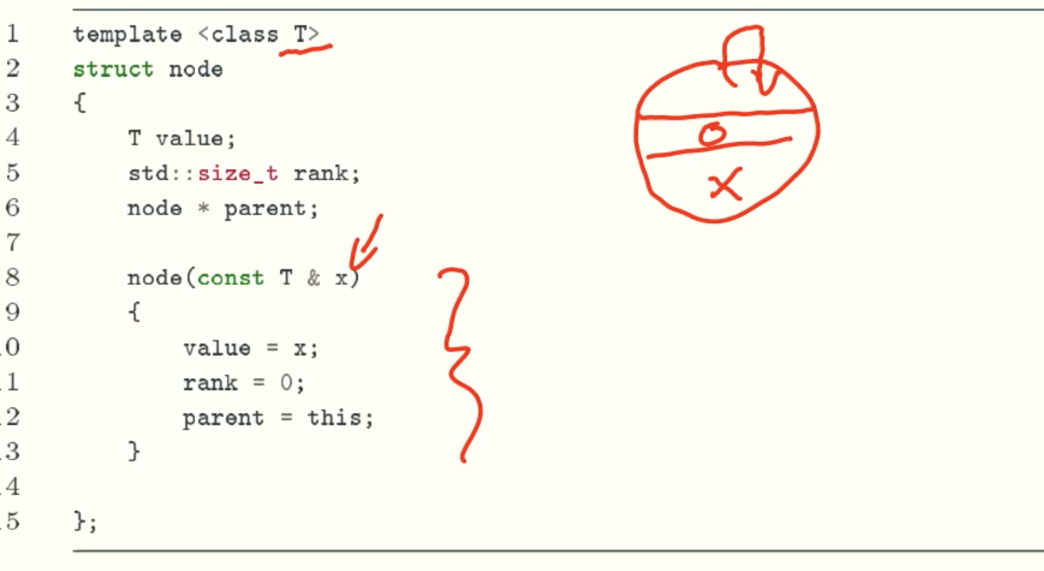
Node

DS

make_set()

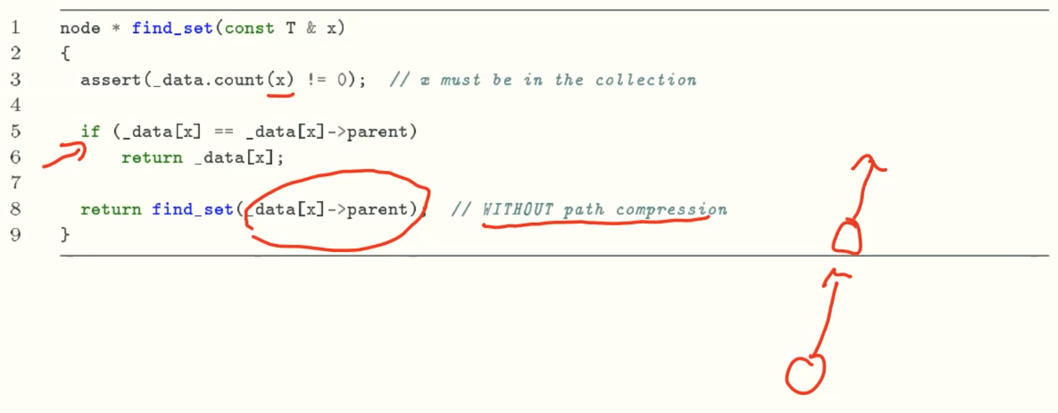
find_set()

join_set()

Application

Kruskal’s algorithm

Example

Analysis

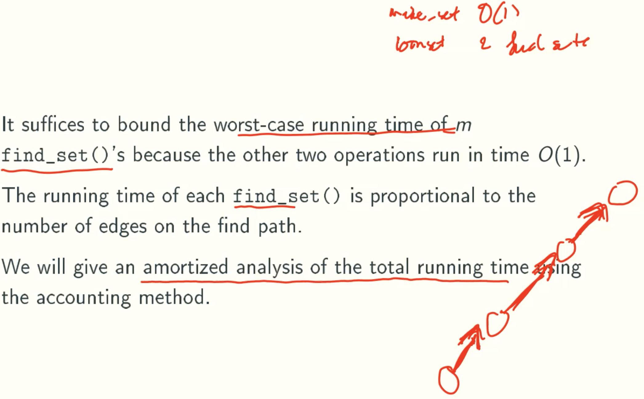
• make_set() and join_sets() runs in time O(1)
• find_set() runs in time O(h), where h is the maximun tree height in the collection
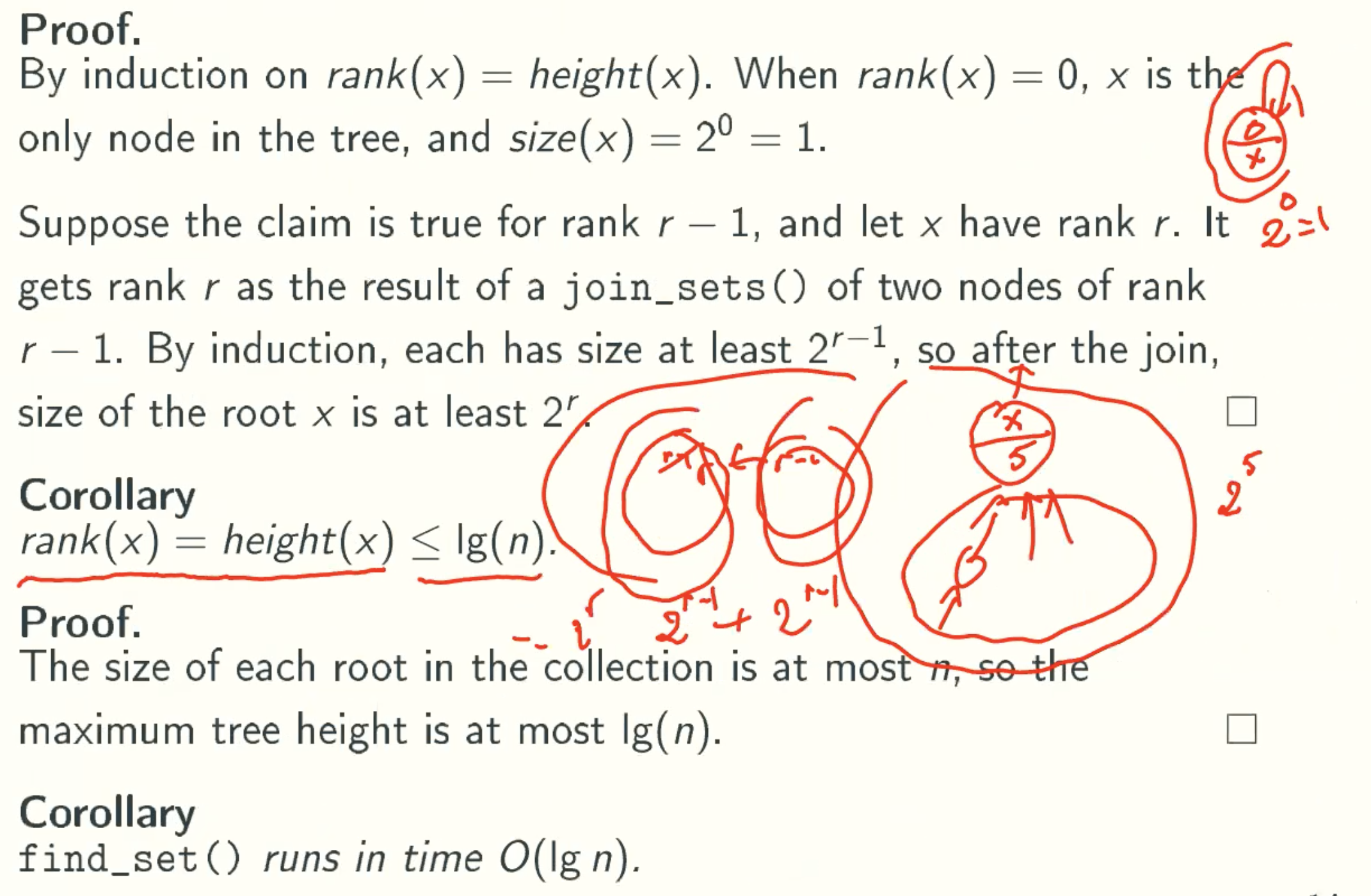
• We will show that h ≤ O(lgn), where n is the total number of nodes

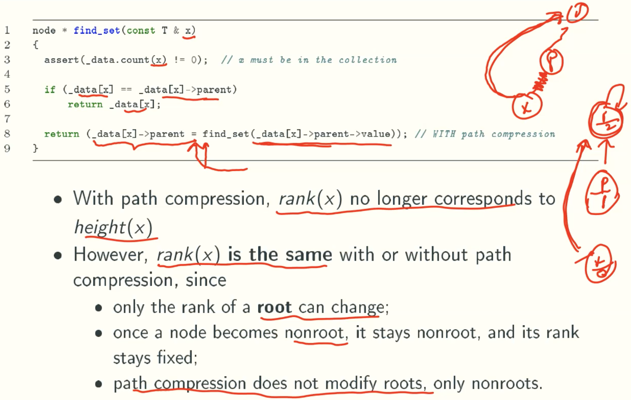
rank(x) = height(x)

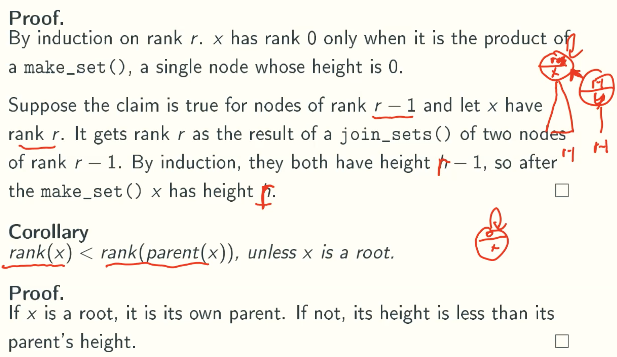
2 ^ rank(x) ≤ size(x)

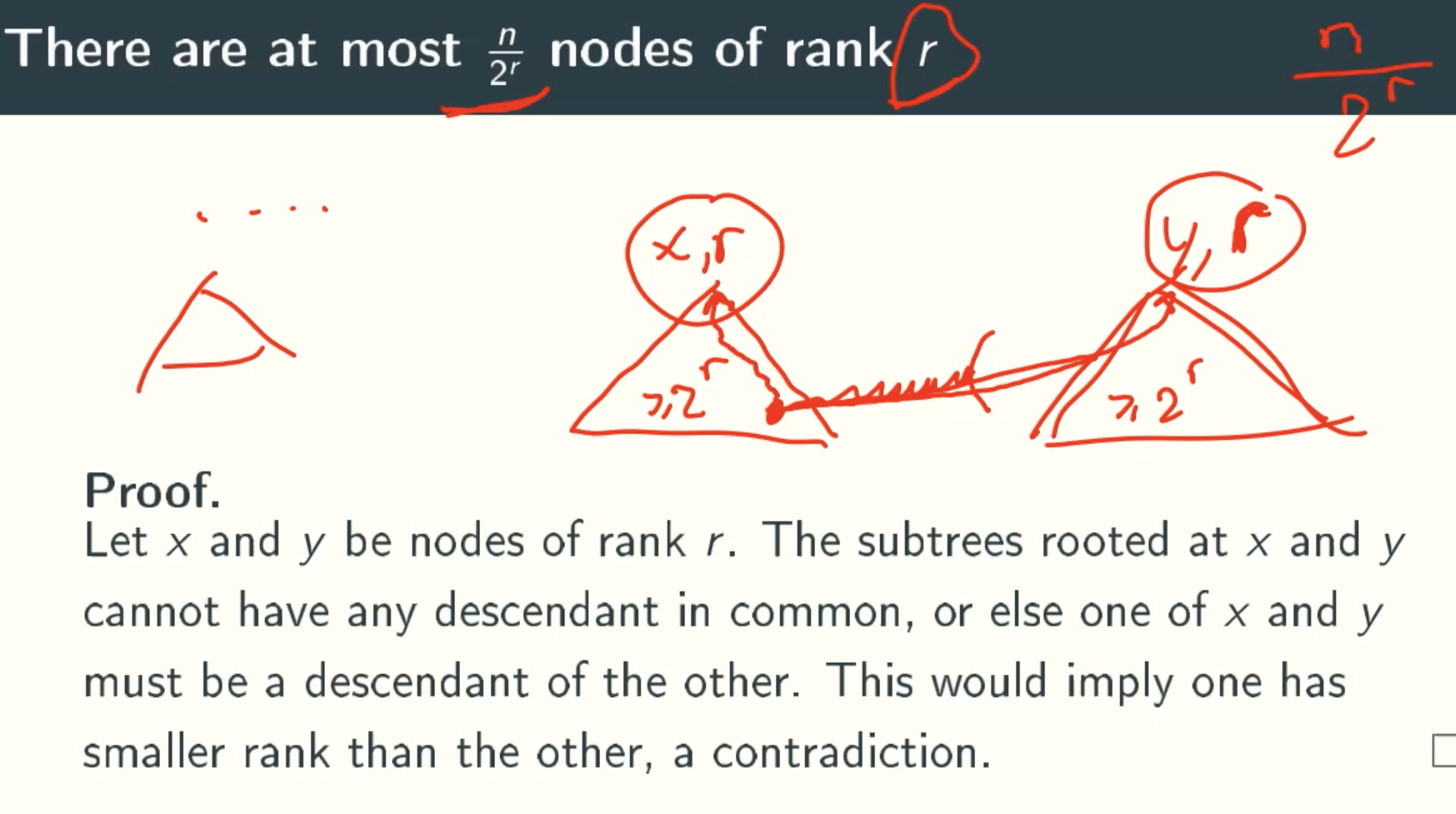
At Most n/2^r Nodes Of Rank r

Path Compression Version

Overview

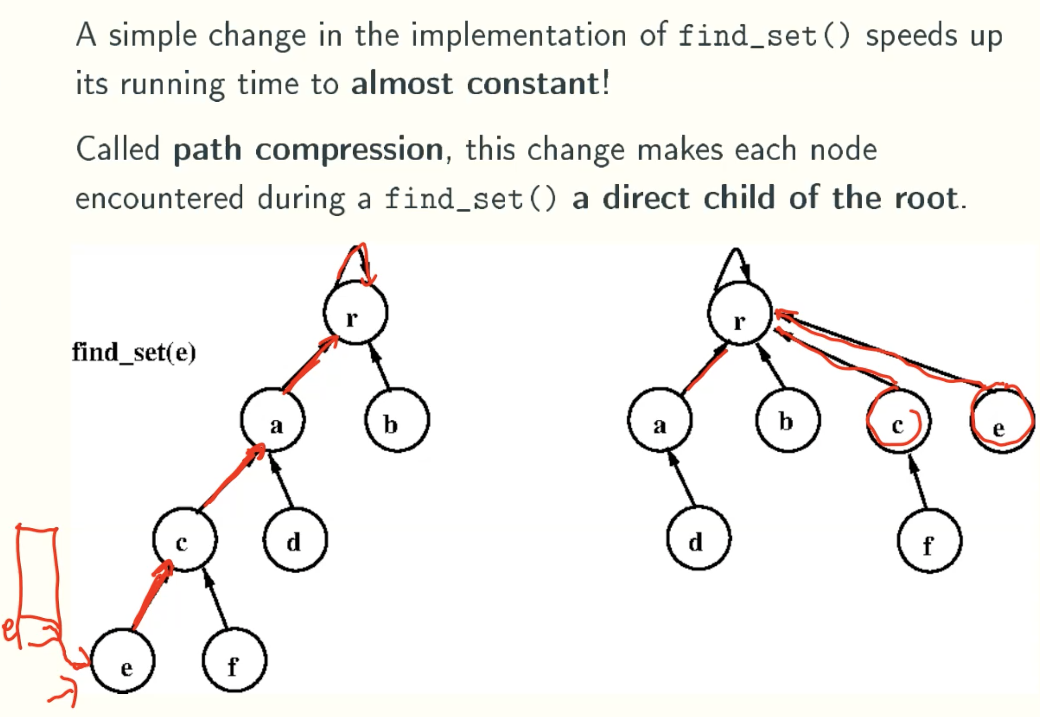
Find_set()

Analysis of path compression

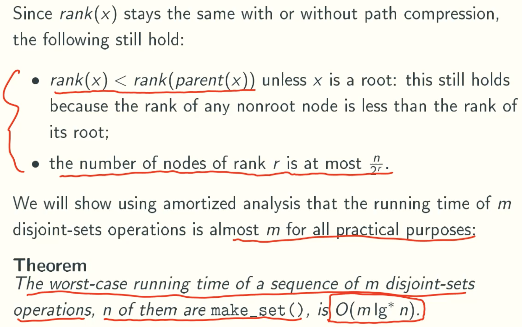
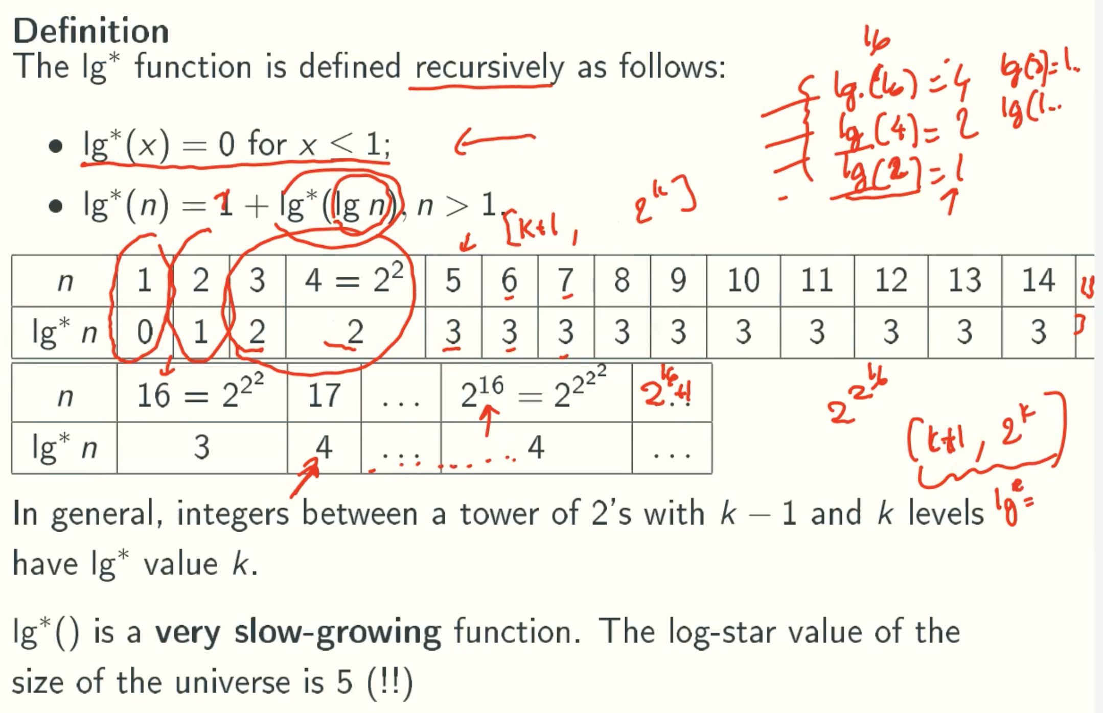
lg*(n) function

Proof

Edge Classification

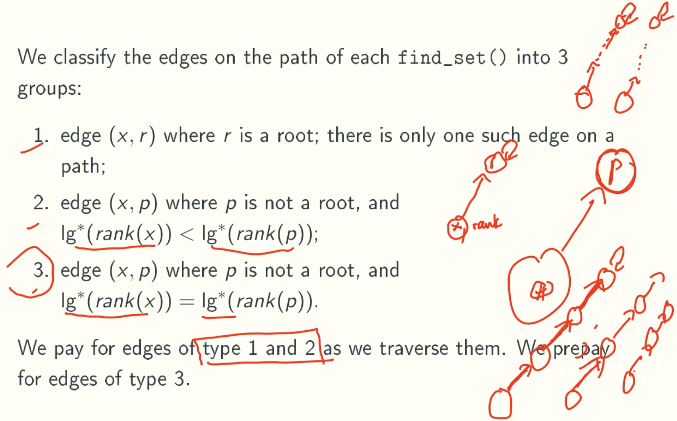
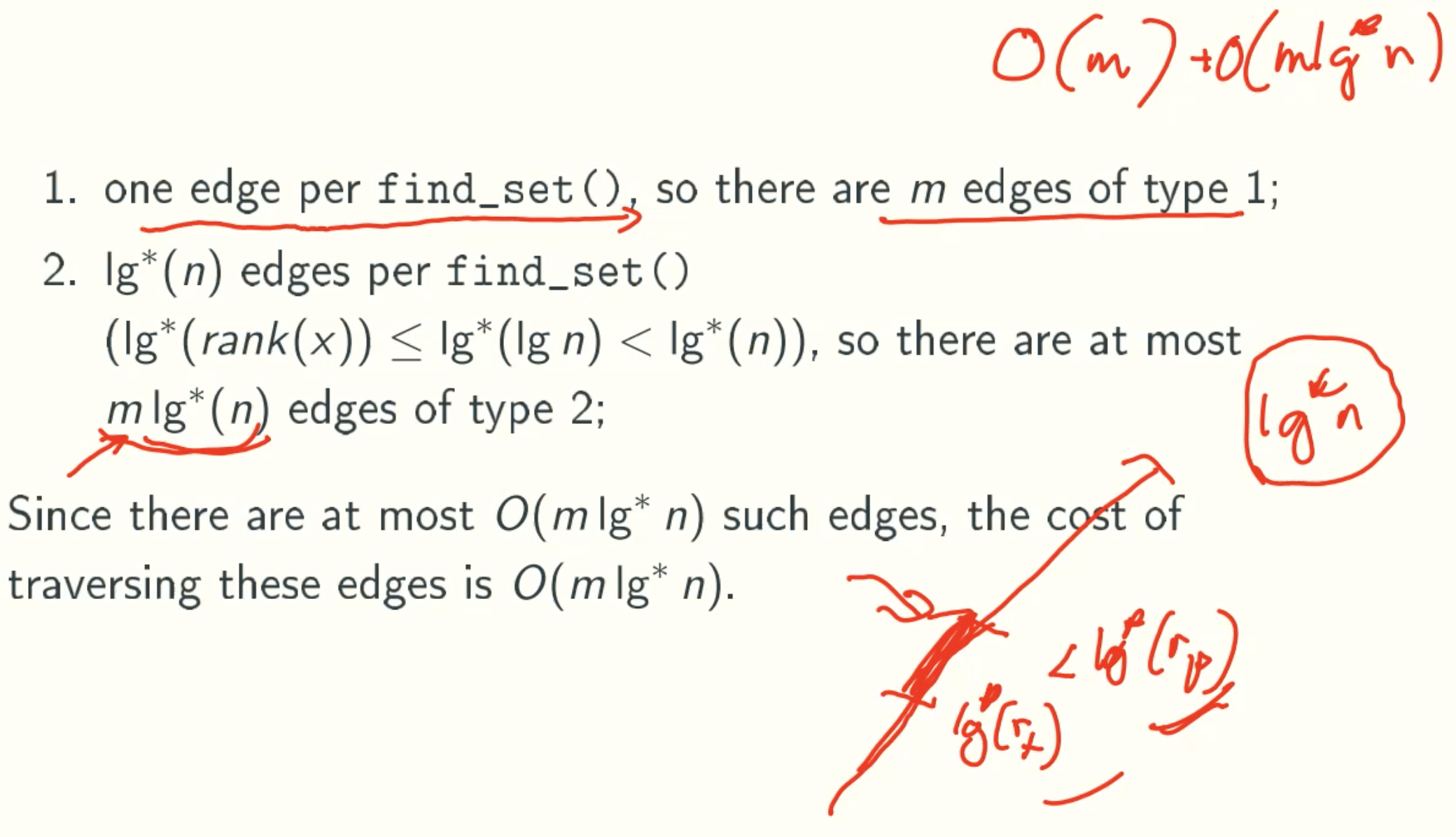
Number of Type1 and Type2

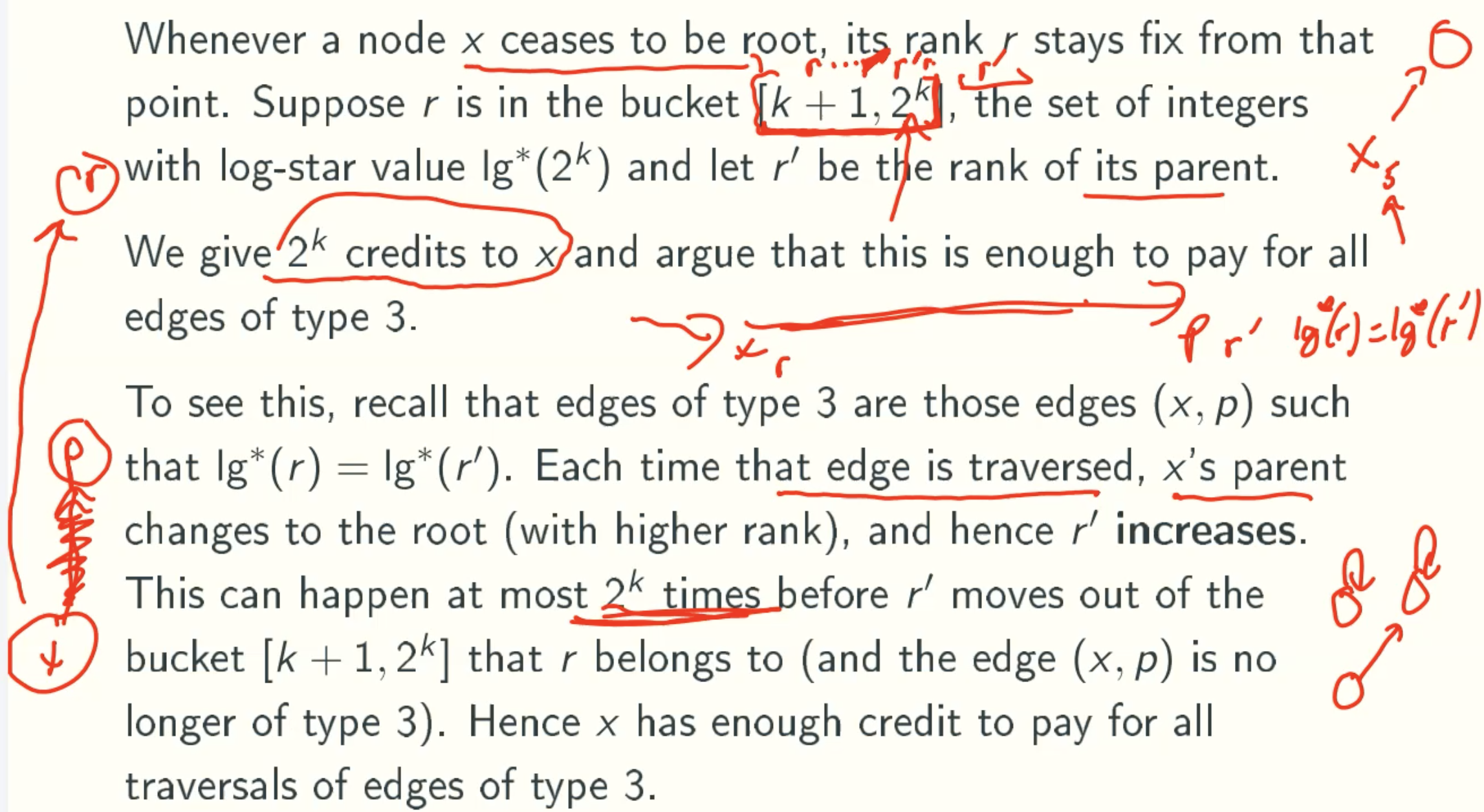
Prepaying for Type3

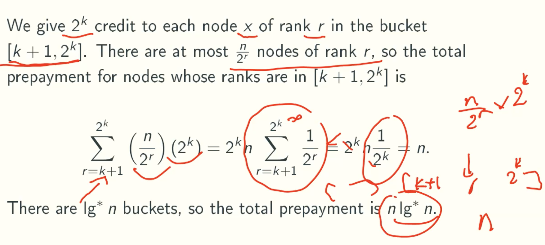
Total Prepayment

Total Running time

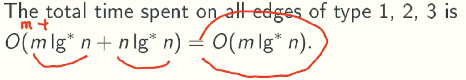
A Tighter Bound Is Possible

Using a more sophisticated prepayment method, it is possible to show that the worst-case running time of m disjoint-sets operations is O(m𝓪(m,n)), where 𝓪(,) is the inverse Ackermann function, as even slower-growing function.

Heap

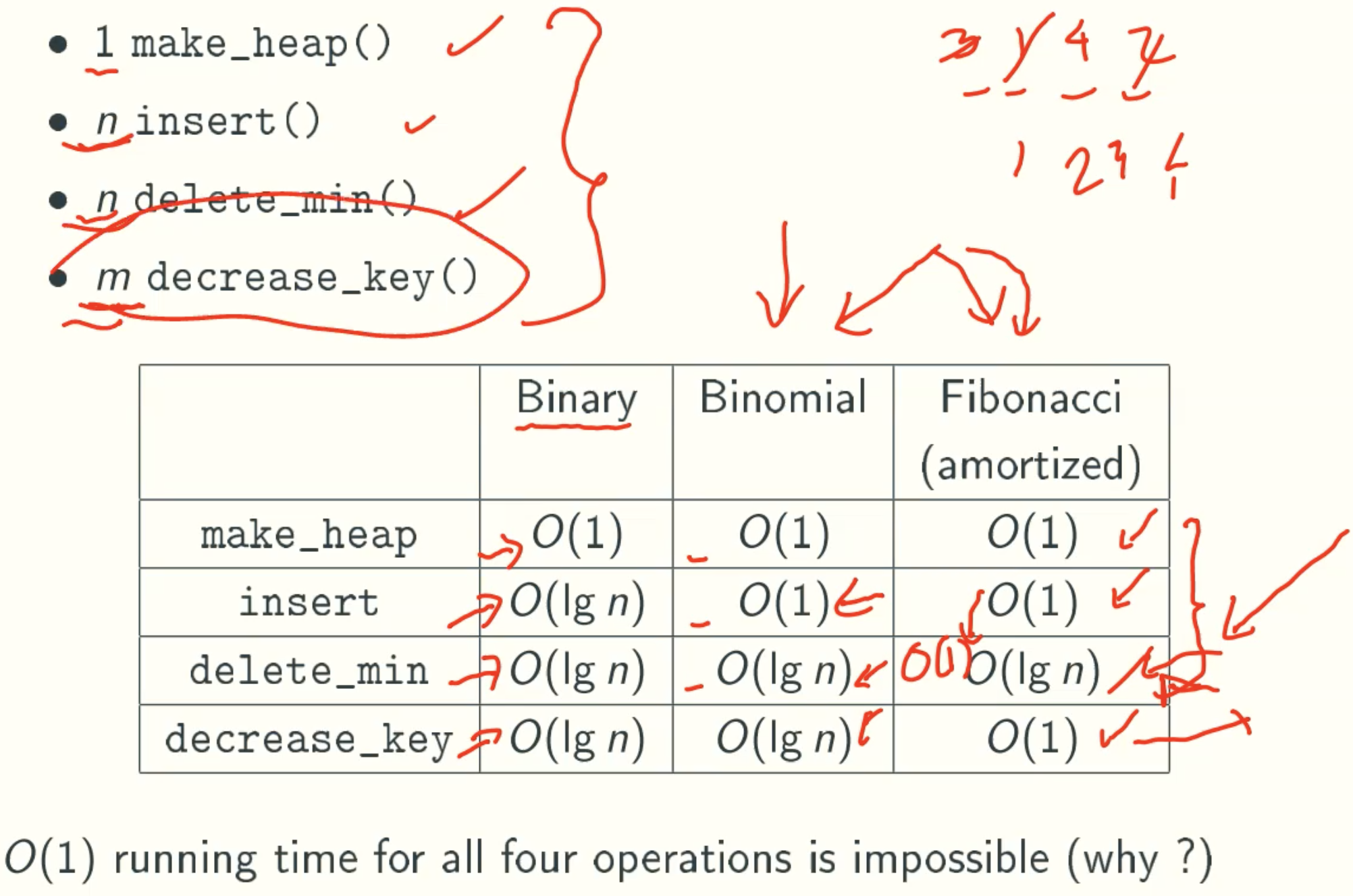
Prim’s Algorithm Based On Heap

Analysis

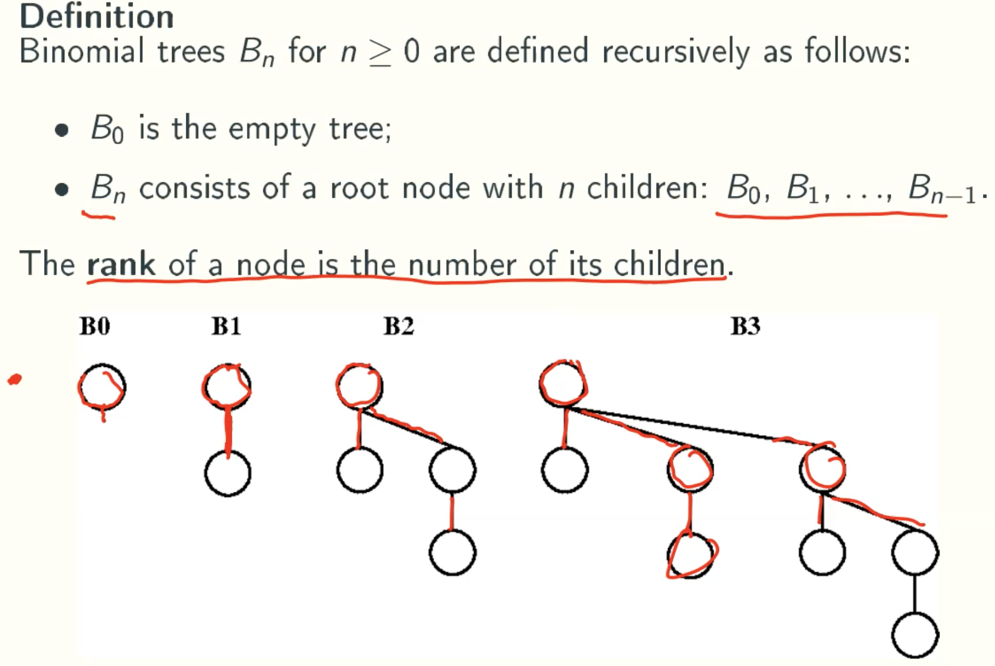
Binomial Heaps

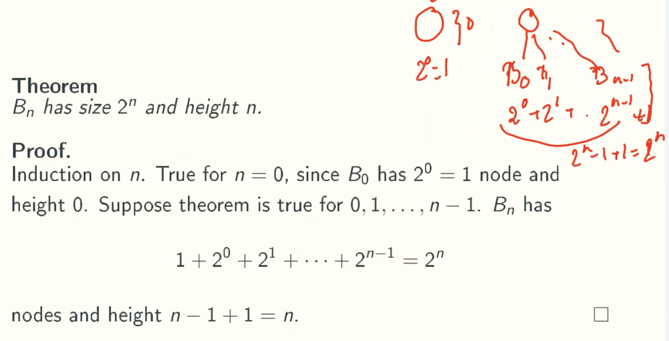
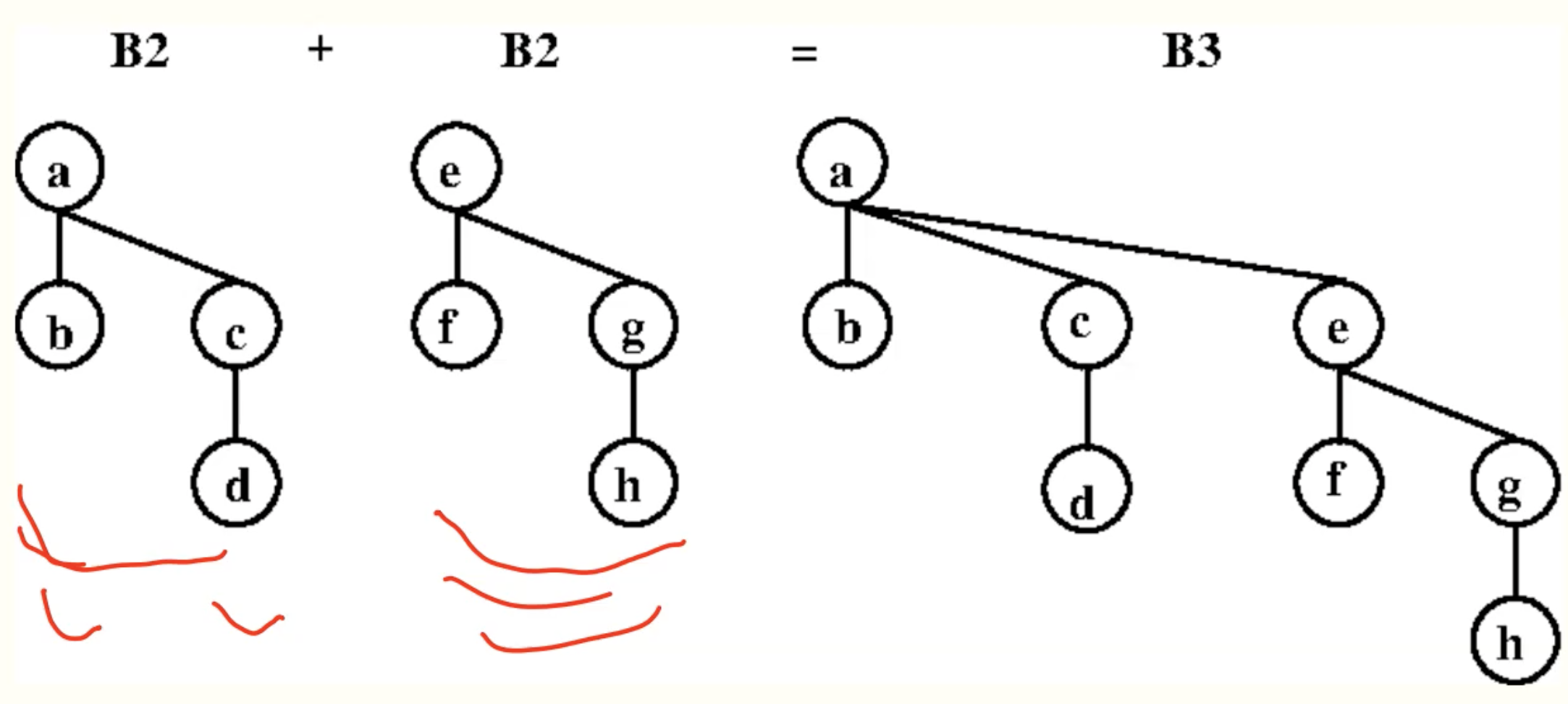
Binomial Trees

Property

Merge

Definition

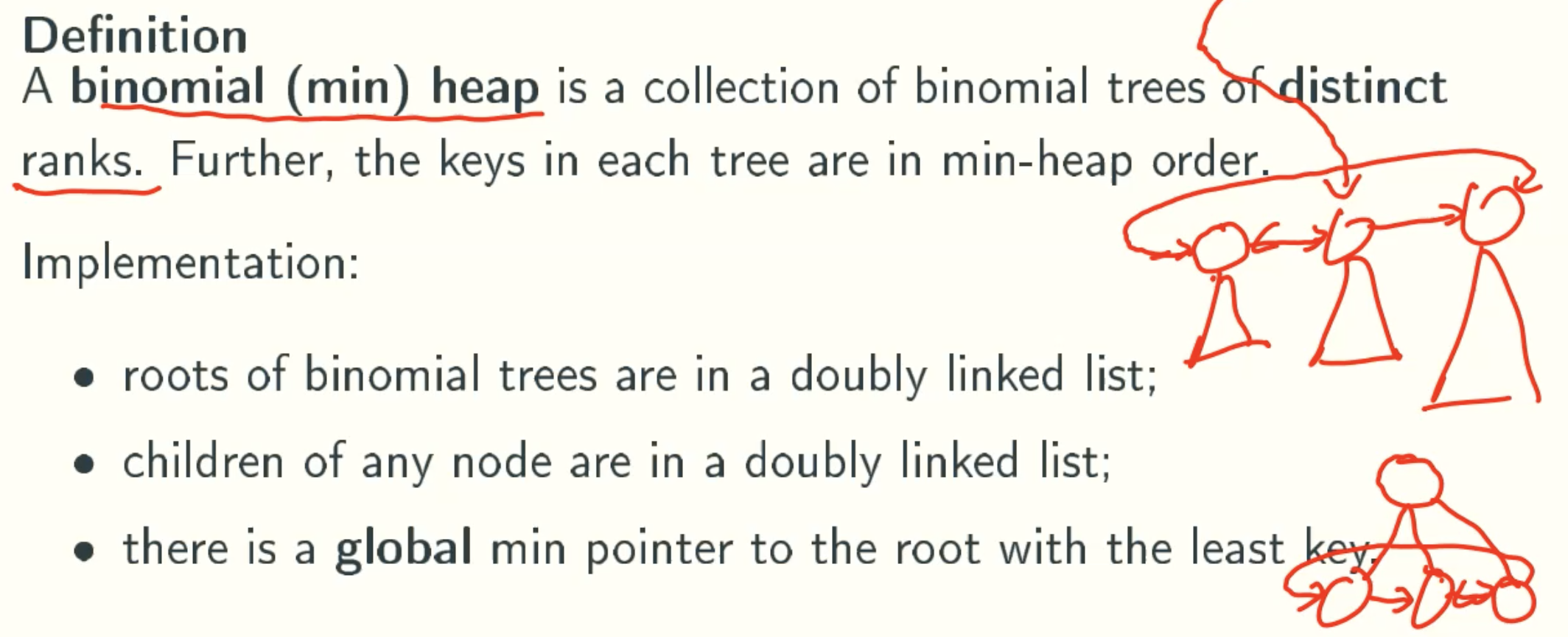
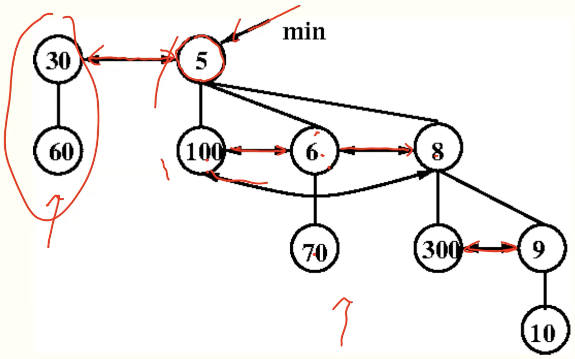
Properties

Let H be a binomial heaps

• H has height at most lgn, since a binomial tree of height k has 2^k nodes;
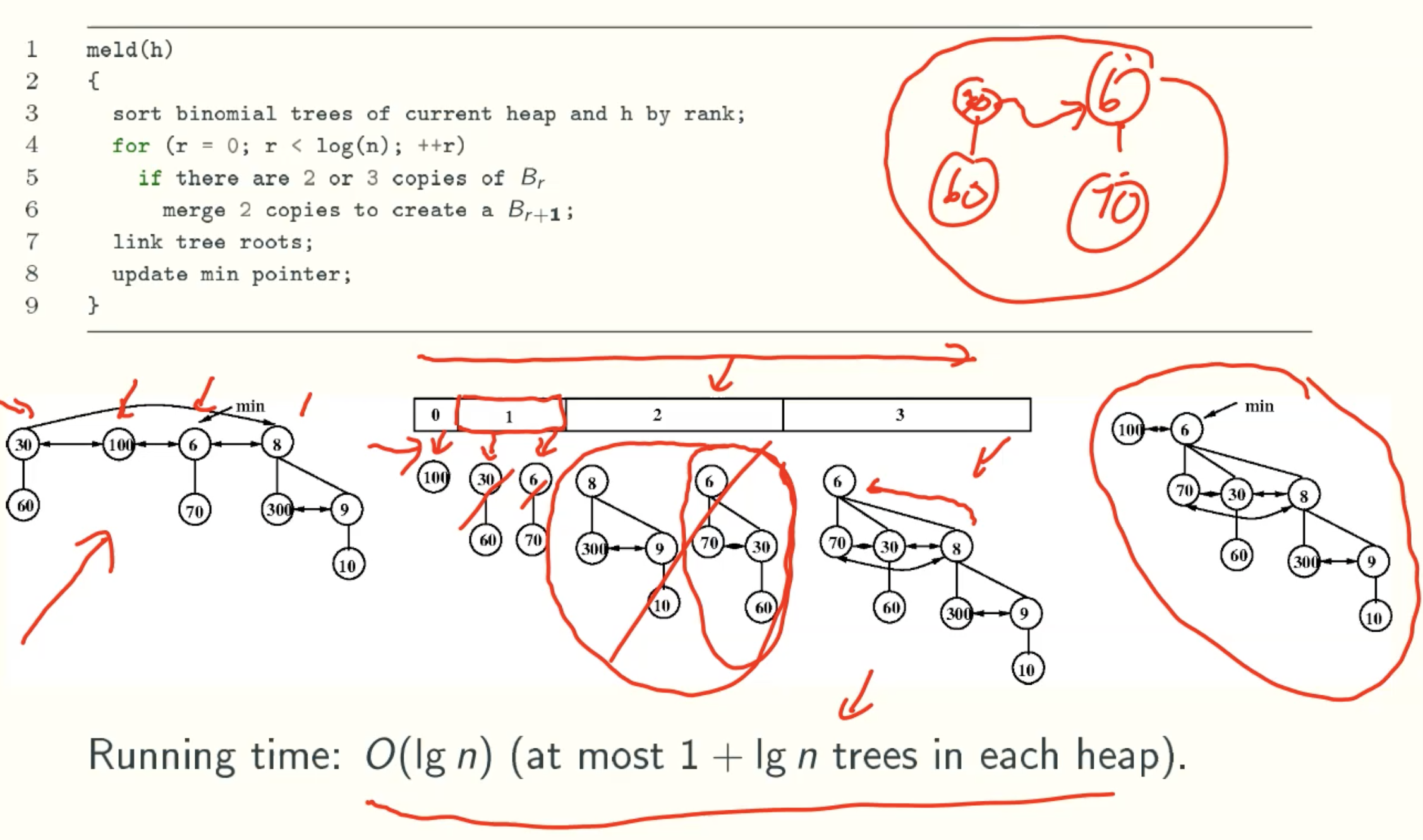
• H has at most 1 + lgn trees, since the trees have distinct ranks at most lgn;
• the rank of each tree in H is at most lgn

Operations

1. make_heap(x): create a heap with a single key;
2. min(): return the minimum key in heap;
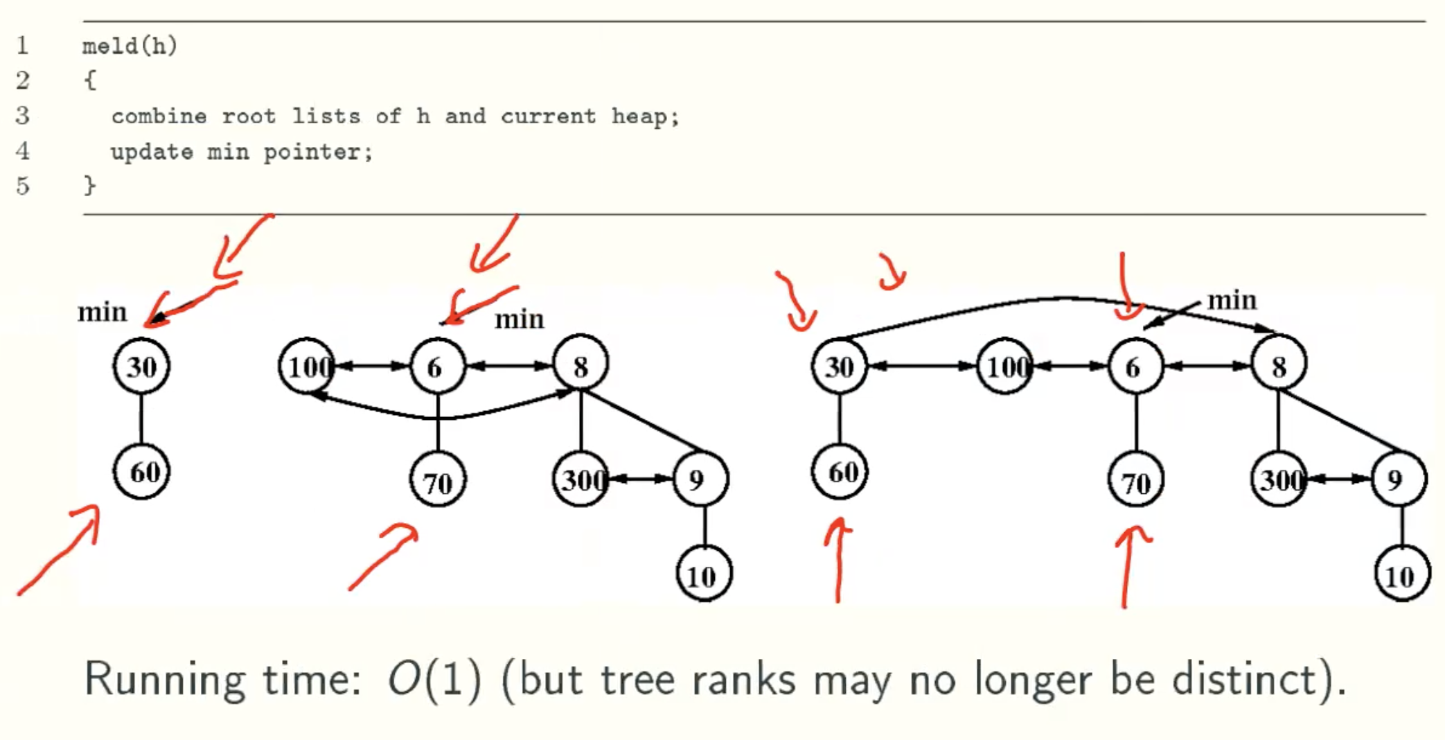
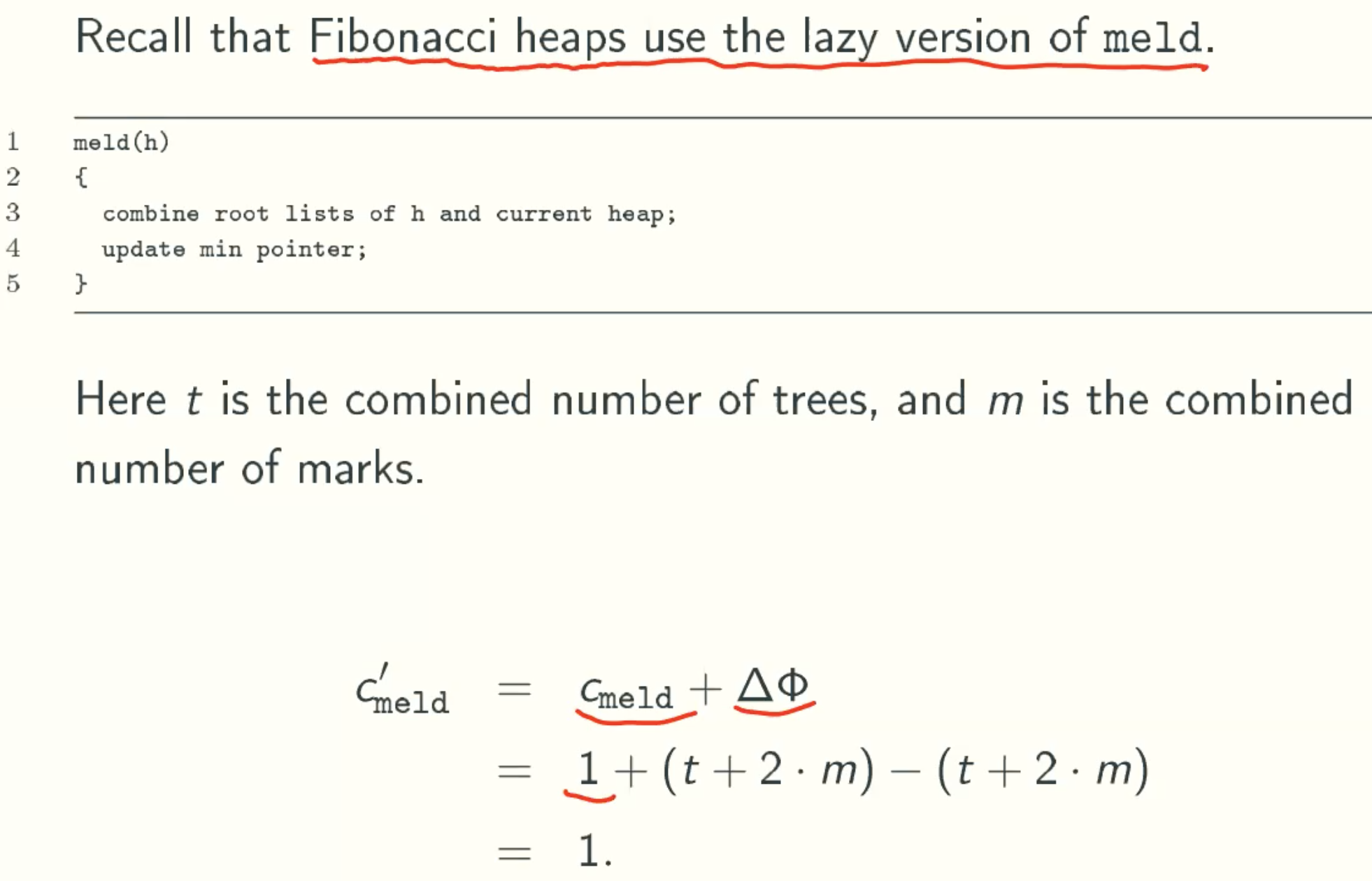
3. meld(h): merge heap h with current heap(h is destroyed);
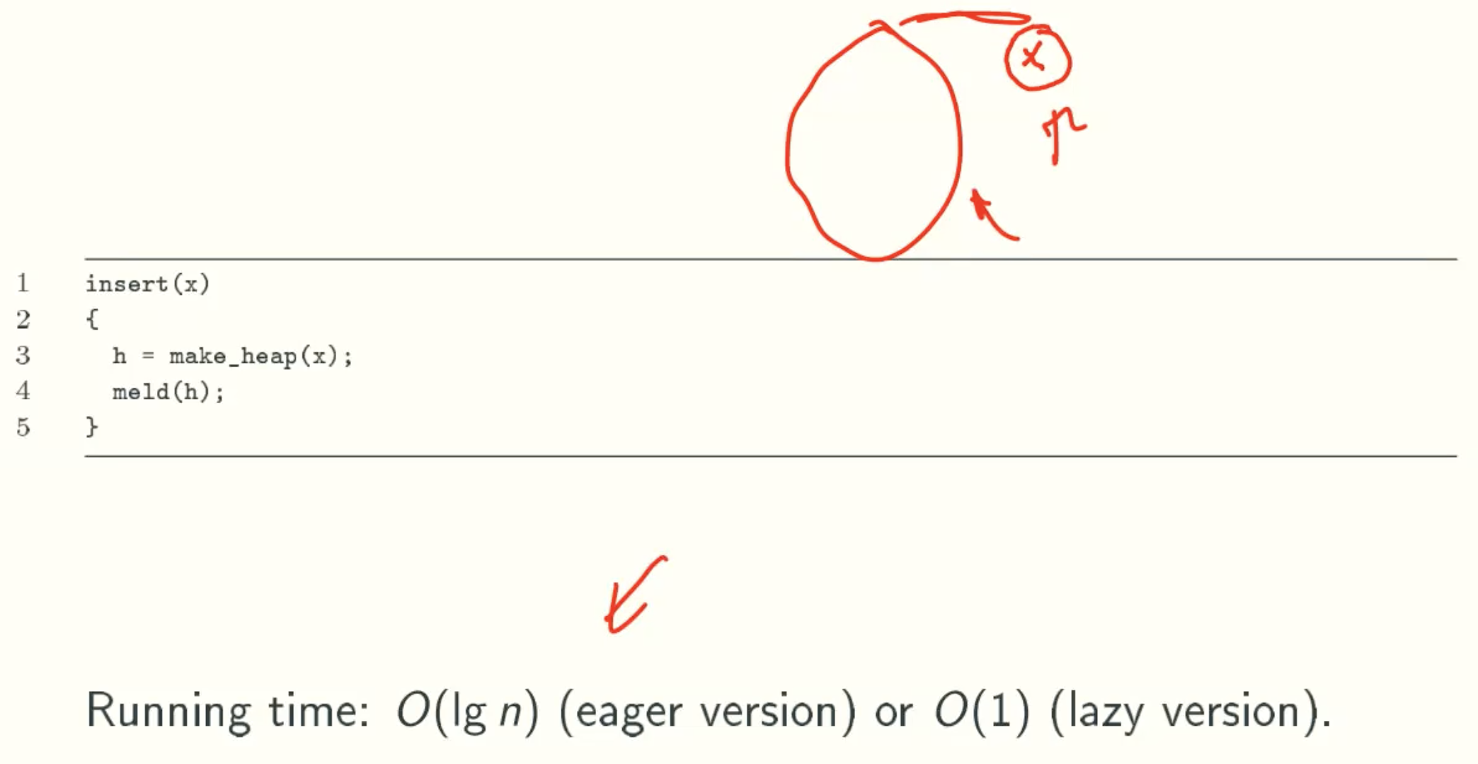
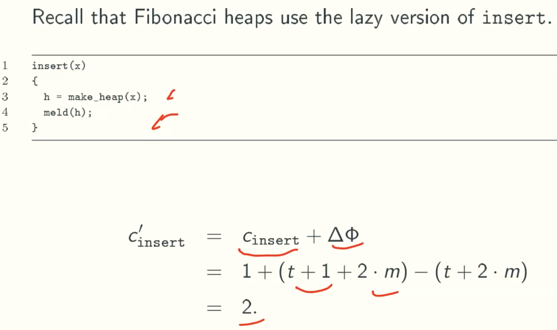
4. insert(x): add key x to current heap;
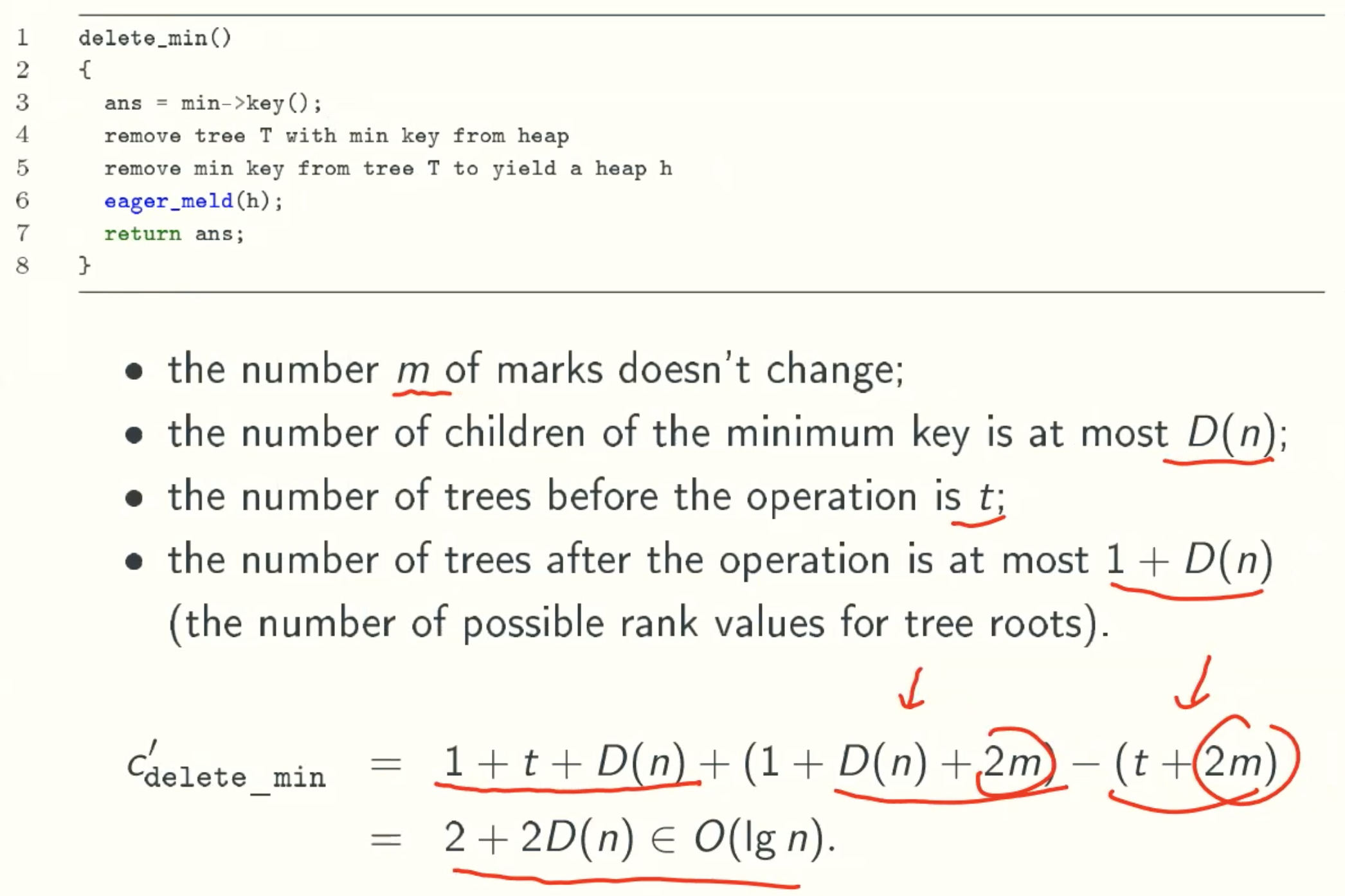
5. delete_min(): remove the minimum key in heap;
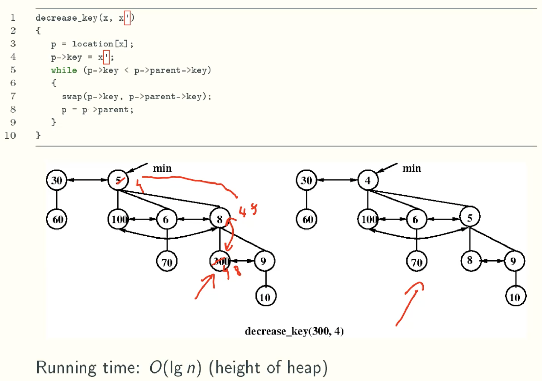
6. decrease_key(x, x’): reduces key x in current heap to x’.

decrease_key(x, x’)

meld(h)

Lazy Version

Eager Version

insert(x)

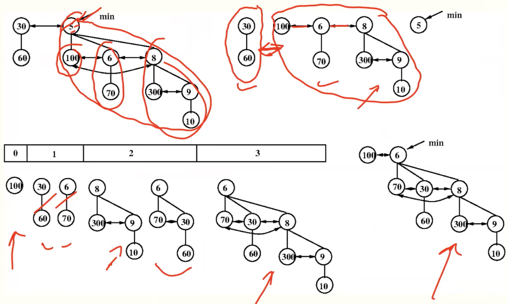
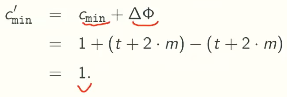
delete_min()

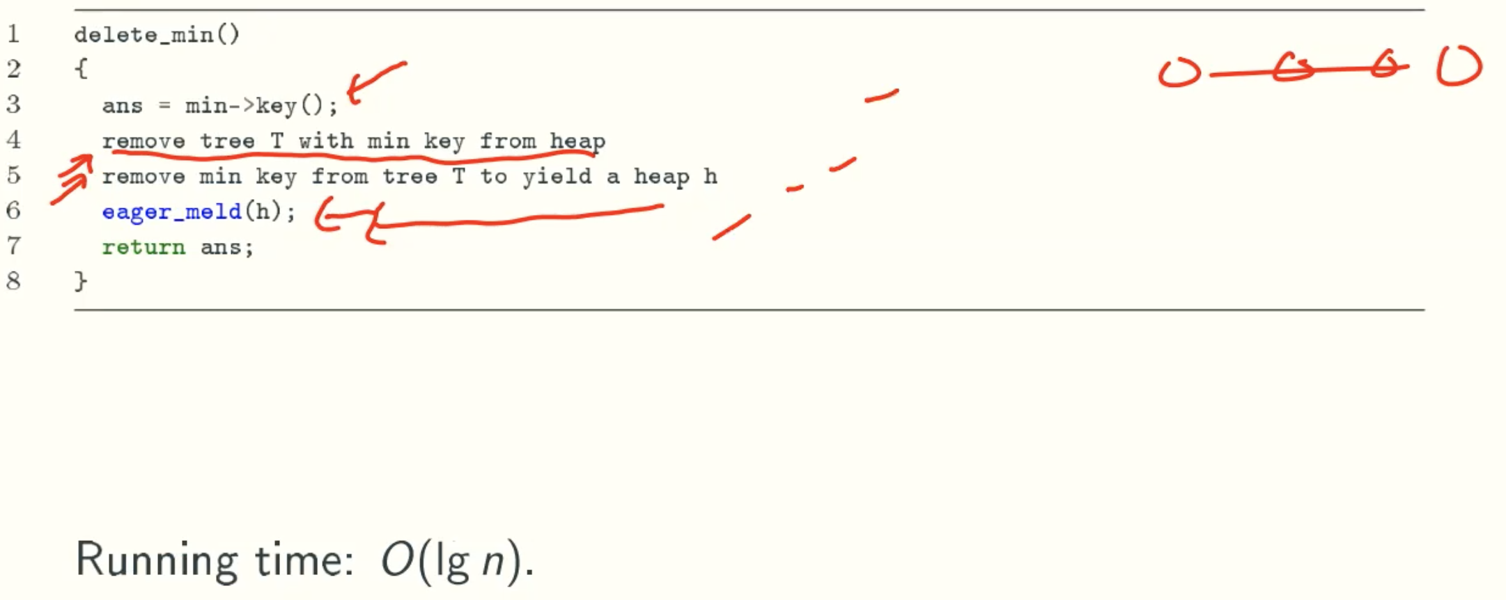
Summary

Operation	Worst Running Time
make_heap	O(1)
min	O(1)
meld	O(lgn) or O(1)
insert	O(lgn) or O(1)
delete_min	O(lgn)
decrease_key	O(lgn)

Fibonacci Heaps

Fibonacci Number

F₀ = 0
F₁ = 1
F_n = F_n-1 + F_n-2, n ≥ 2.
F = {0, 1, 1, 2, 3, 5, 8, 13, 21, …}

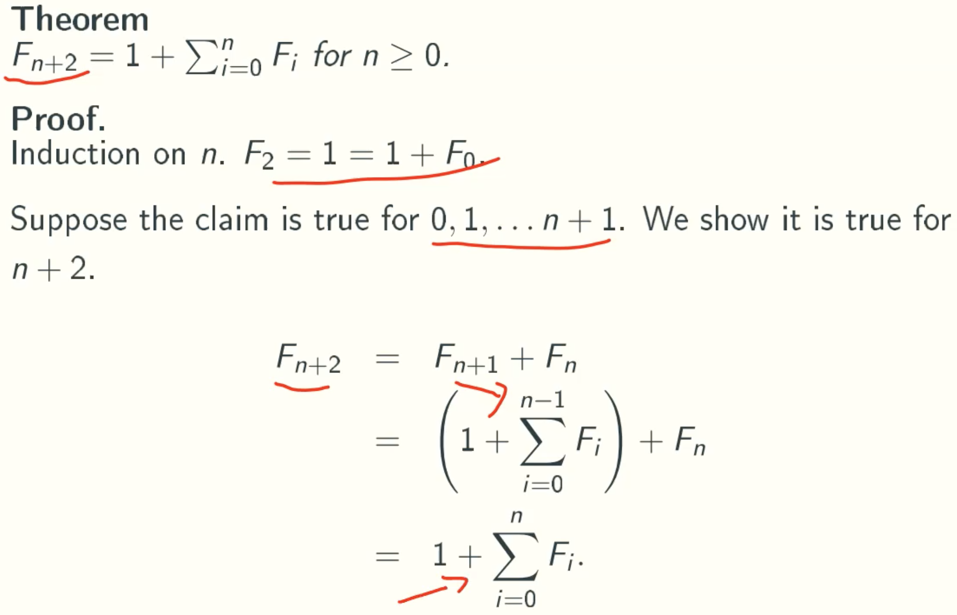
Facts

1. 
2. 

Fibonacci Heaps

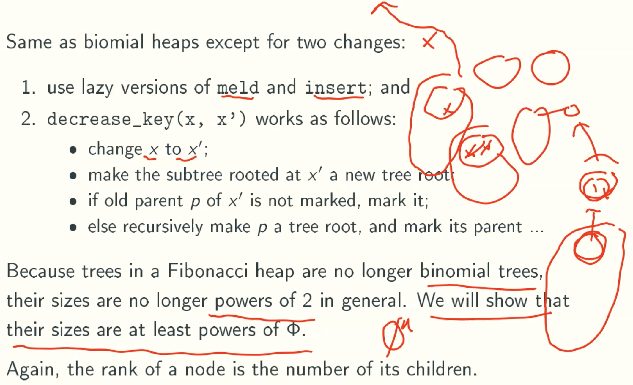
if its parent is root level, not mark its parent.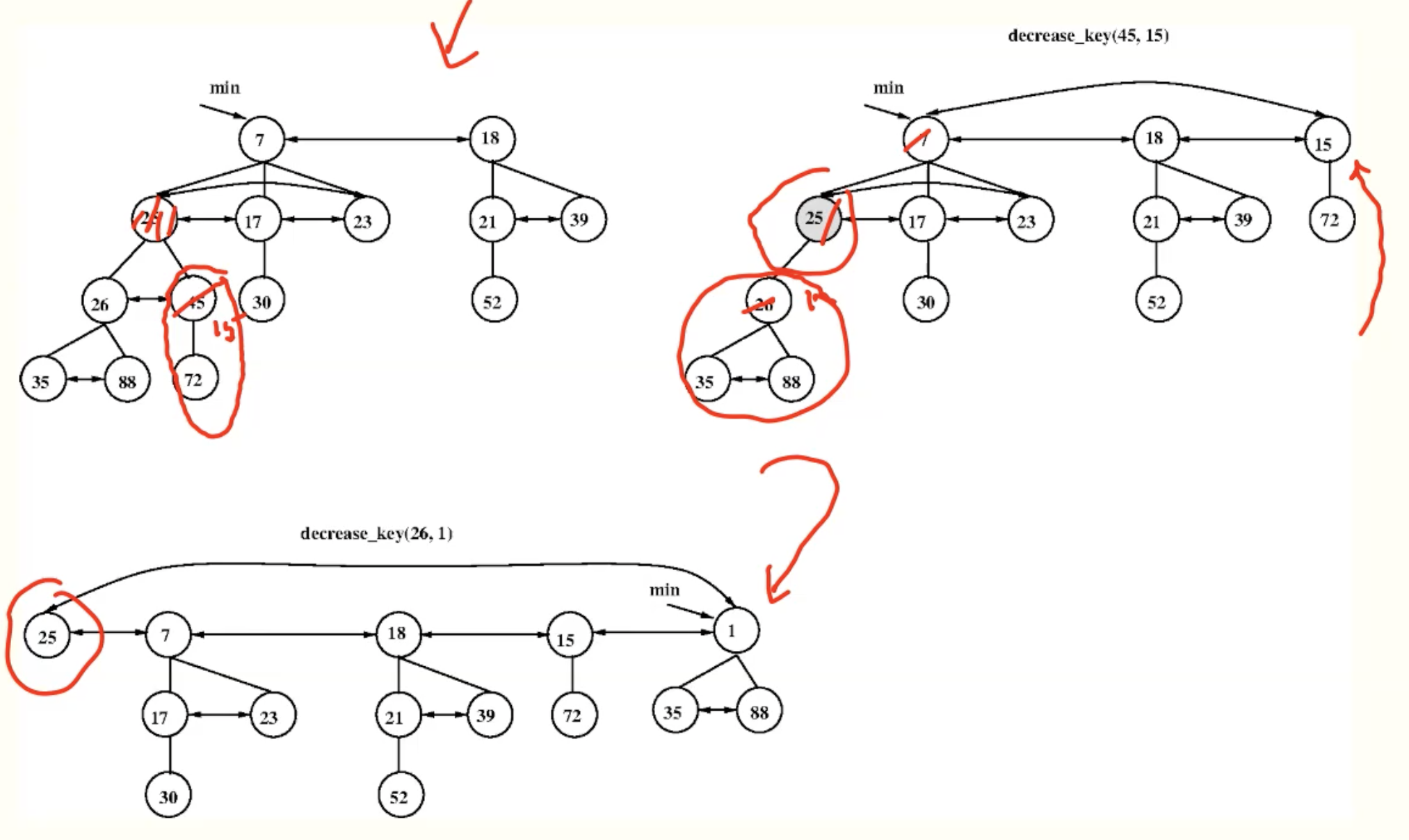

Amortized Analysis

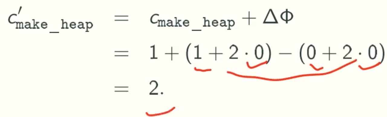
Make_Heap

Min

Meld

Insert

Delete_min

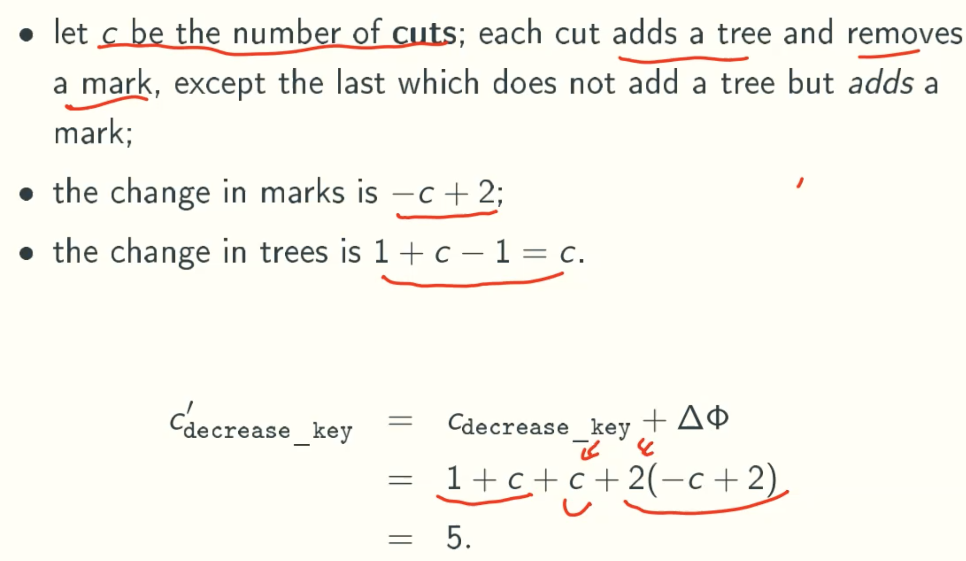
Decrease_key

Summary

Operation	Worst Running Time
make_heap	O(1)
min	O(1)
meld	O(1)
insert	O(1)
delete_min	O(lgn)
decrease_key	O(1)

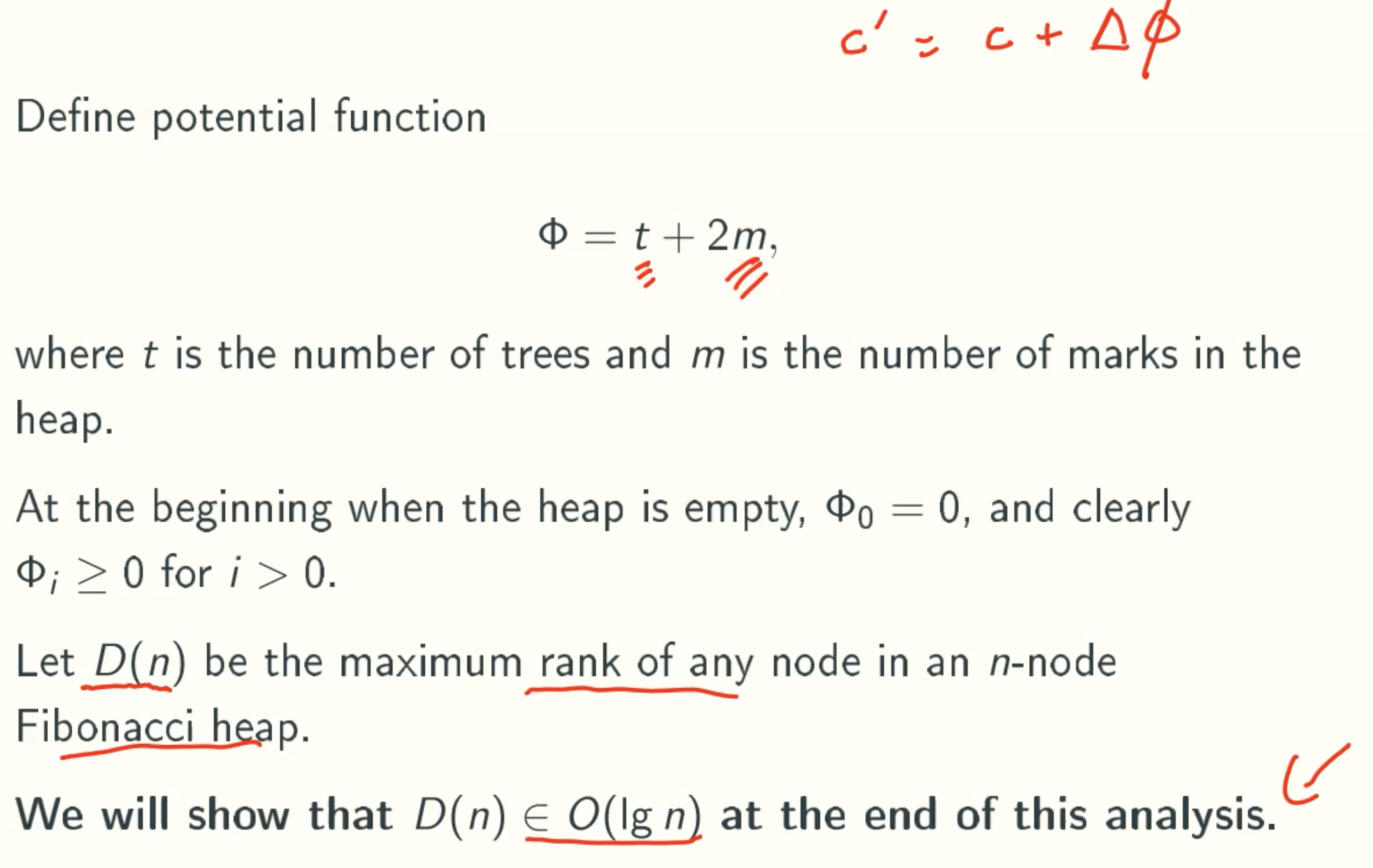
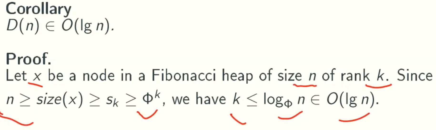
D(n) ≤ O(lgn)

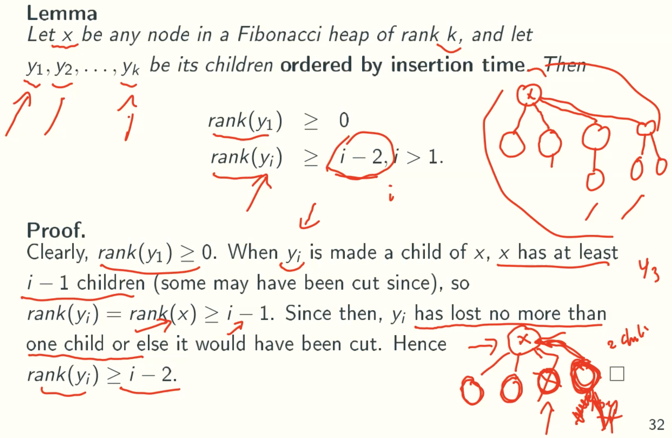
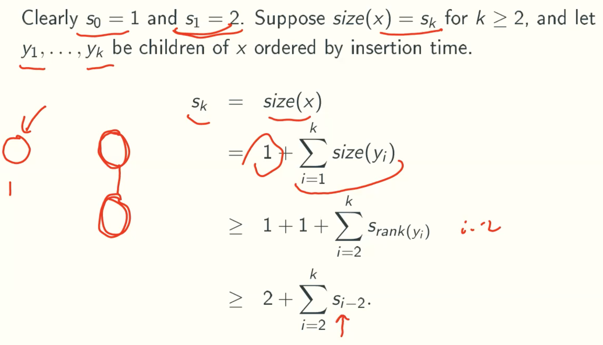
S_k: minimum tree size rooted at a node of rank k

Let size(x) be the number of nodes in the subtree rooted at x, including itself, and let s(k) be the minimum value of size(x) for node x of rank k in any Fibonacci heap.

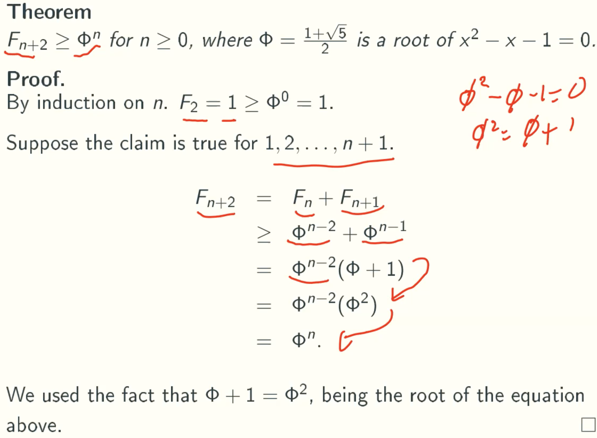
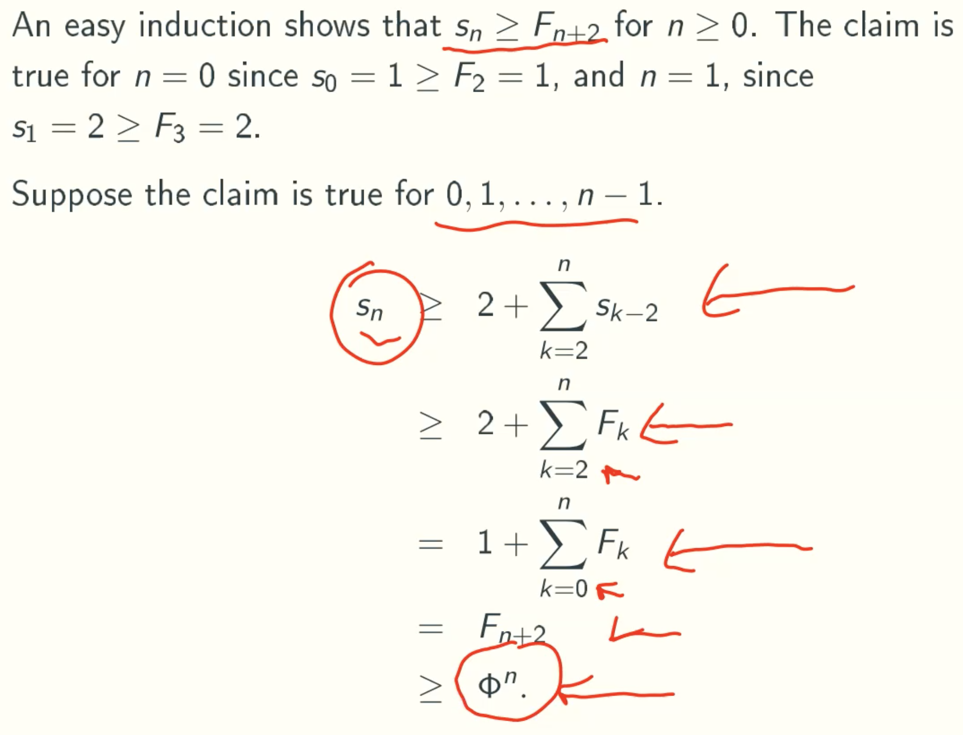
S_k ≥ F_k+2 ≥ Φⁿ

Corollary

String Matching Problem

Definition

Exhaustive Search

Smart Solutions

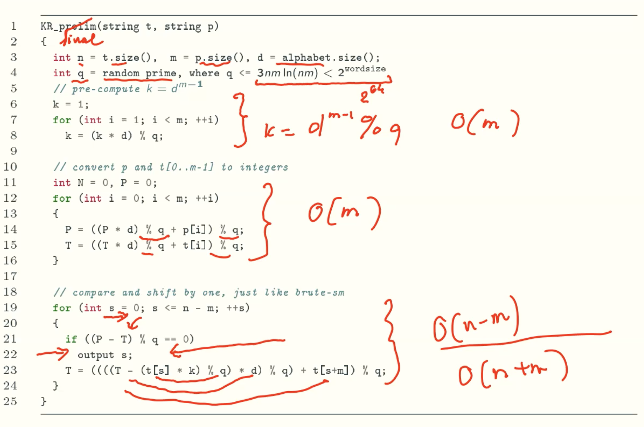
Karp-Rabin

Overview

• consists of Compare-Shift phases as brute-force method;
• always shifts by one;
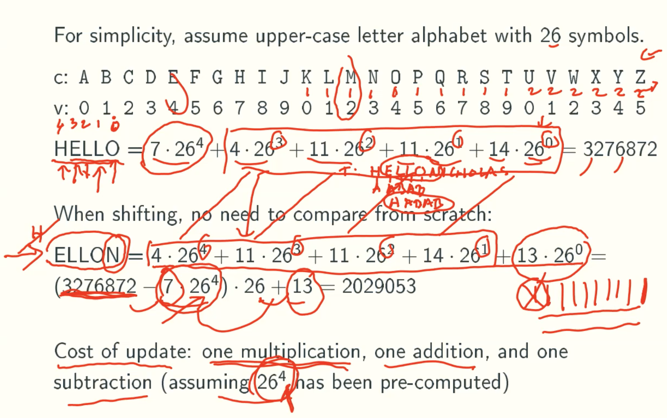
• speeds up compare by treating strings as integers in base d, where d is the alphabet size;

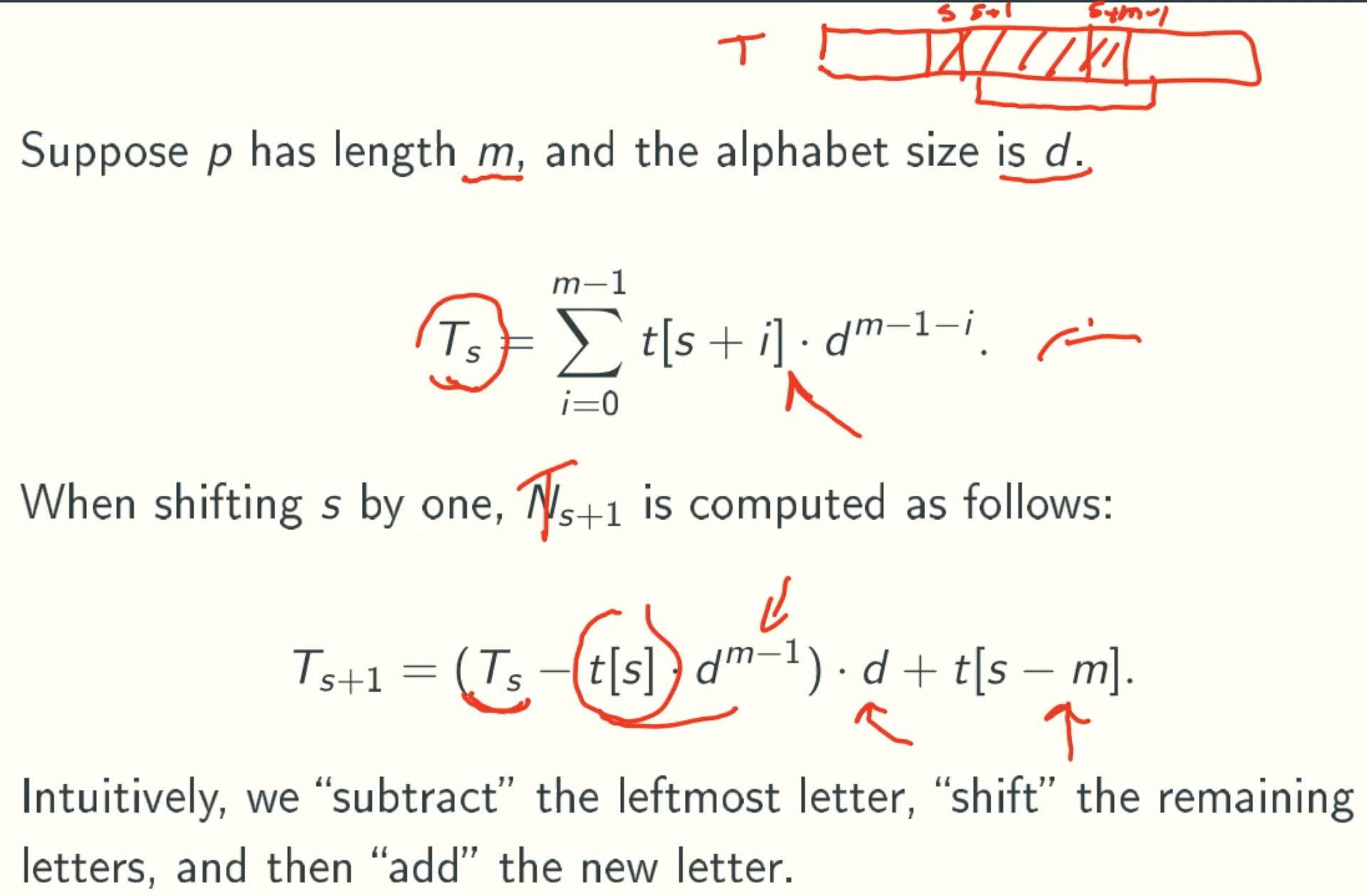
  String as Integer

  
  

Code

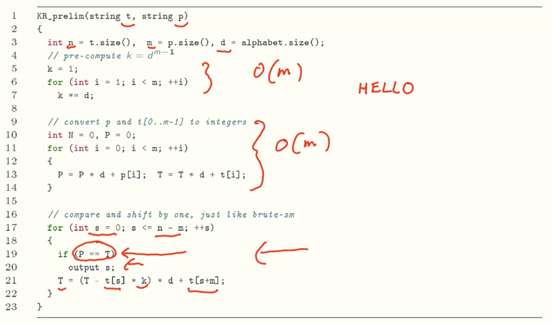
Analysis

θ(m)+θ(n)+θ(n) = θ(n+m) arithmetic operations
Each arithmetic operation cost Ω(m) (integers have size m)
So the total time is Ω(nm), no better than brute-force!

New Ideas

Idea #1

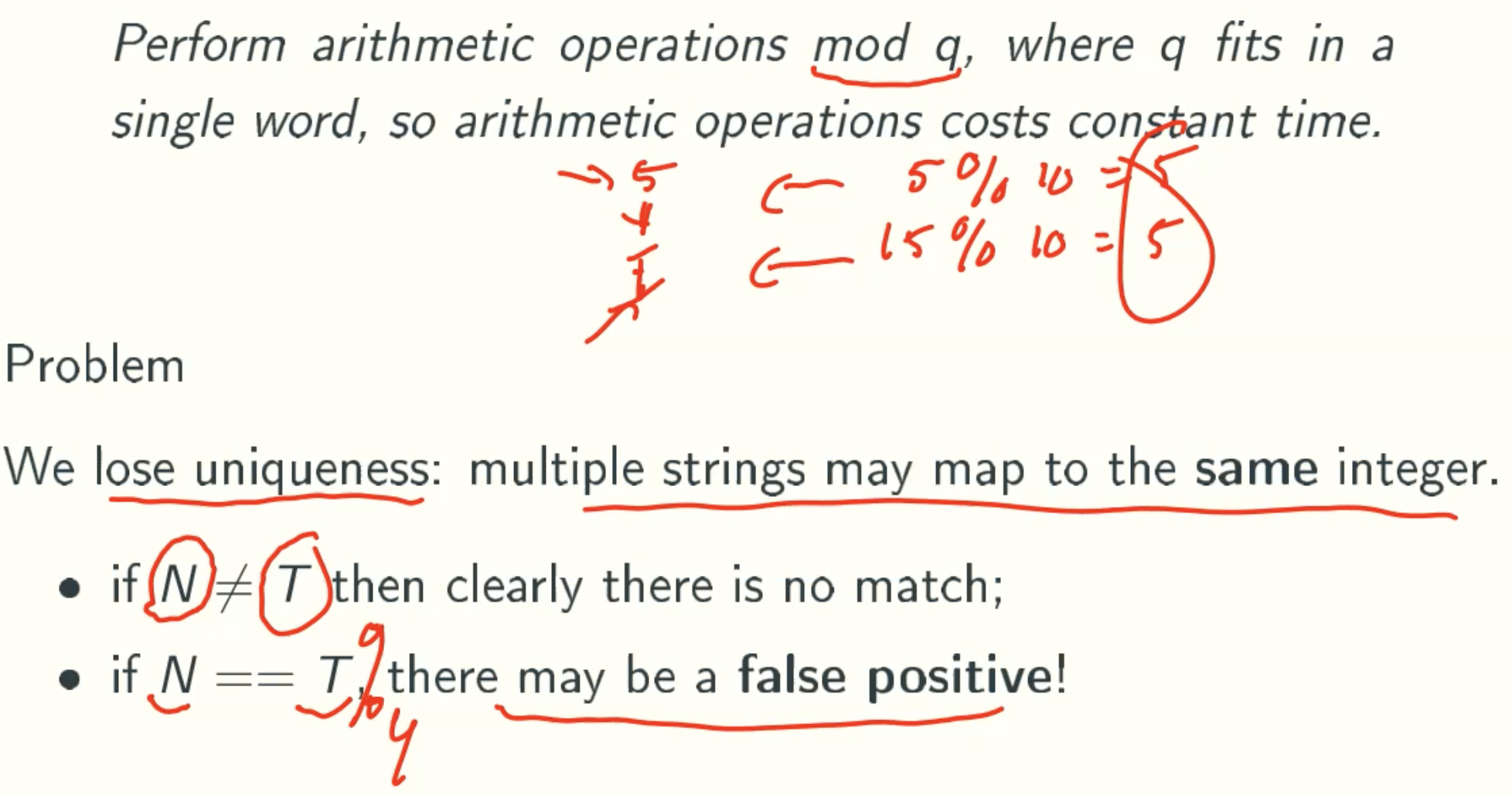
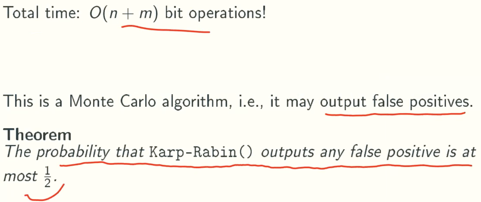
Modification
Accept false positives but keep the error probability negligible using randomization, just like miller-rabin().

Code

Analysis

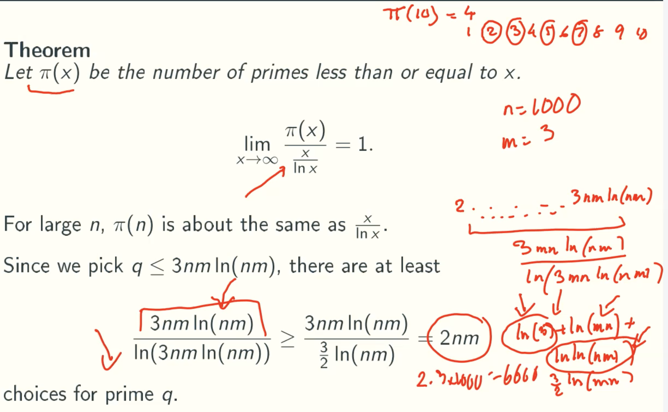
Prime Number Theorem

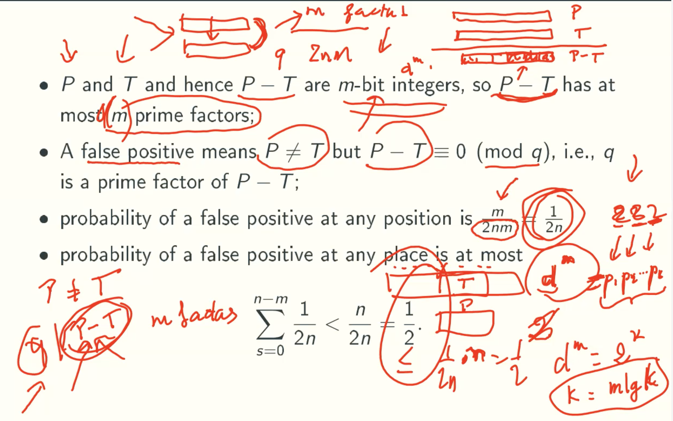
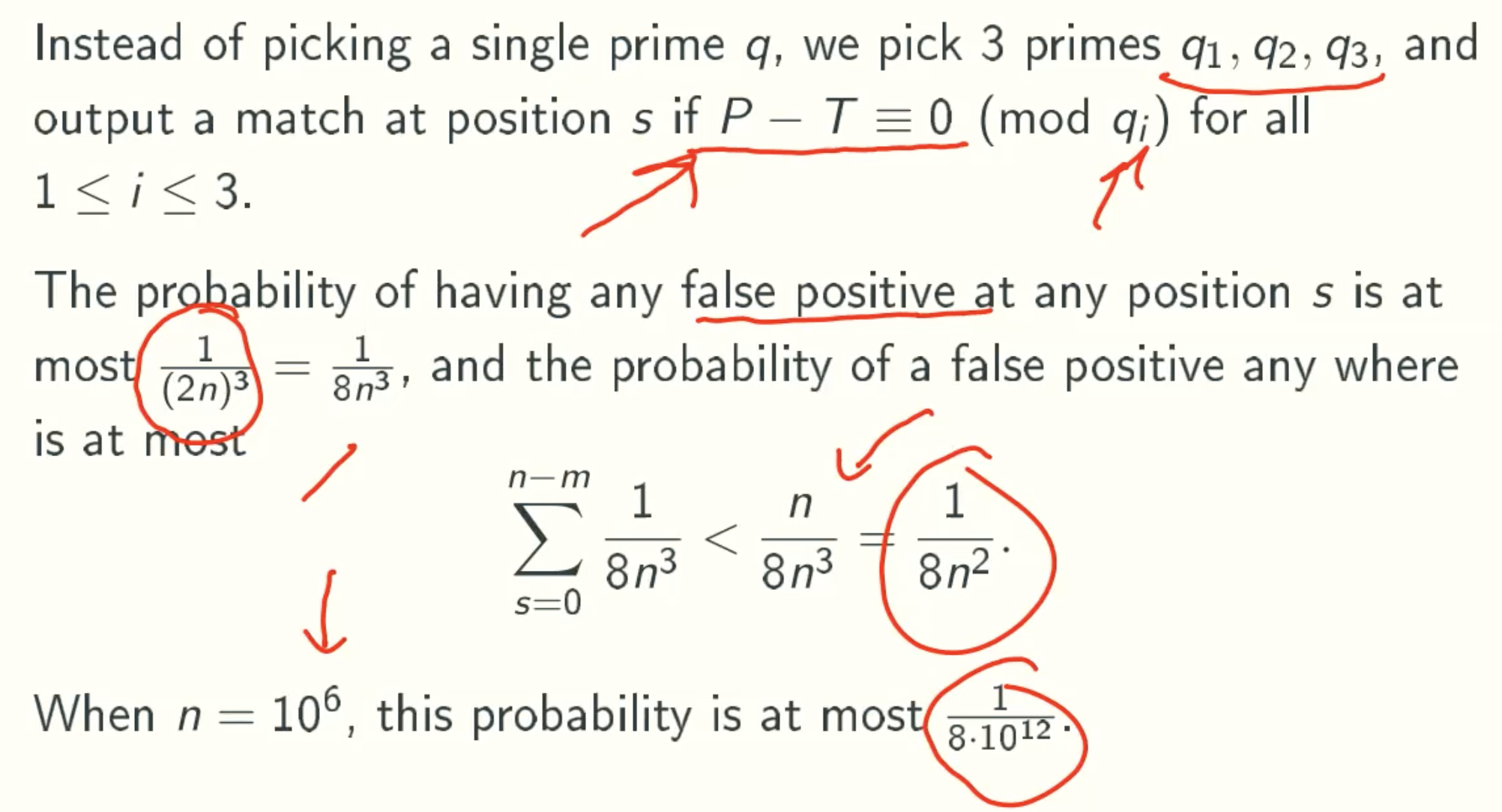
Proof of error bound

Amplification

Fundamental Pre-processing: Z-Values

Overview

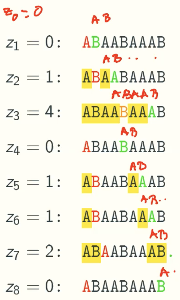
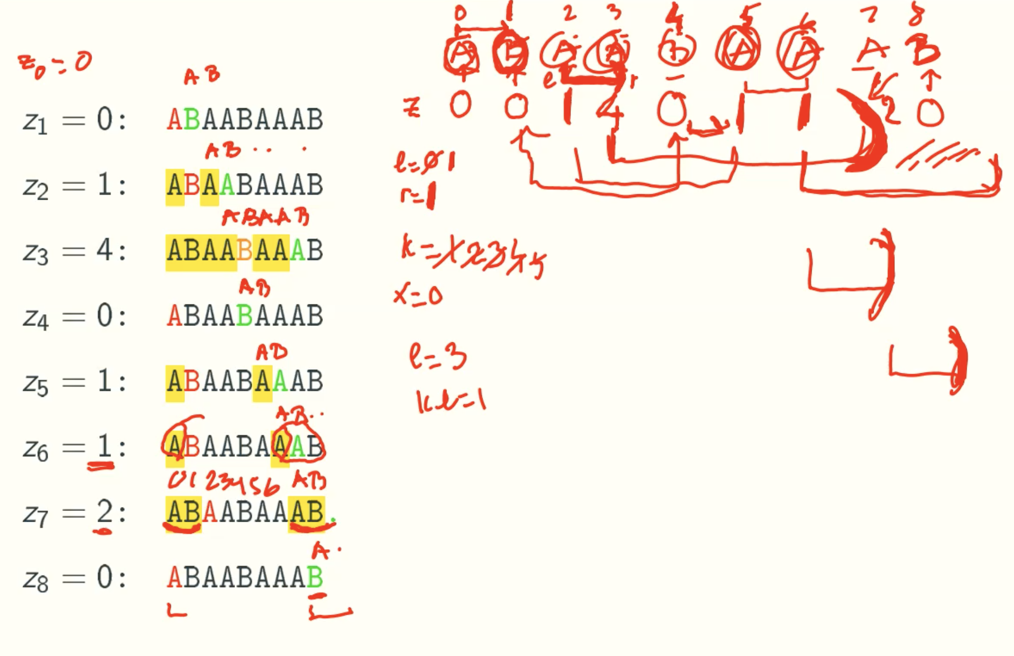
Z-values

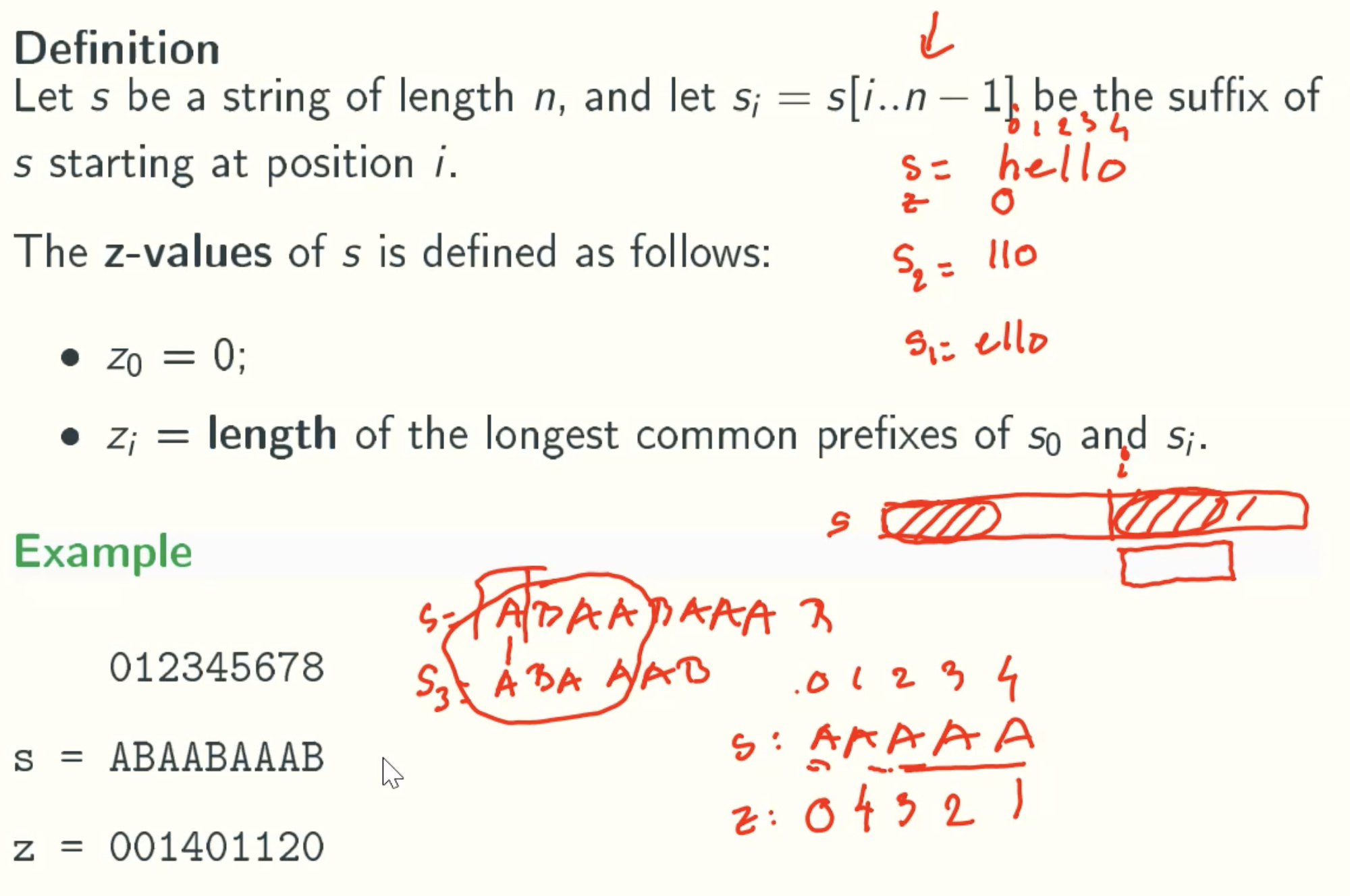
In Details

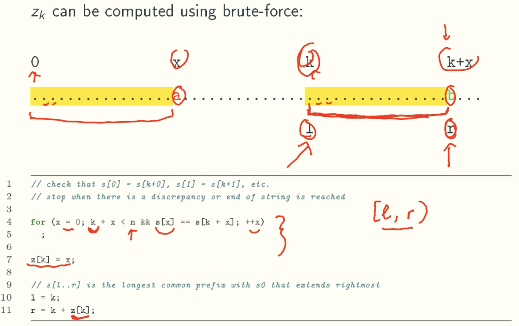
Computing z-values In Linear Time

case 1: Brute Force

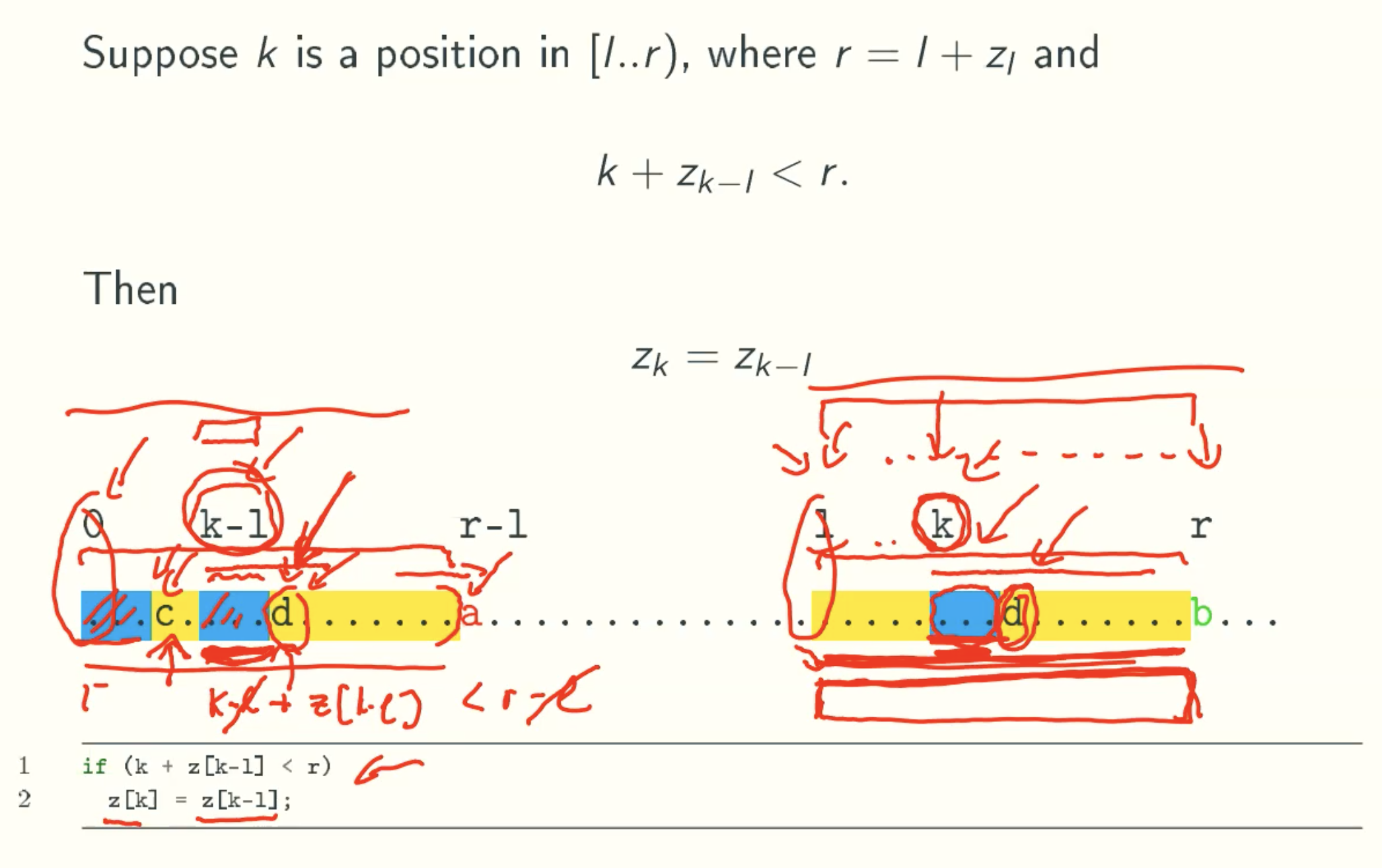
case 2: deducing Zk from a previous z-value

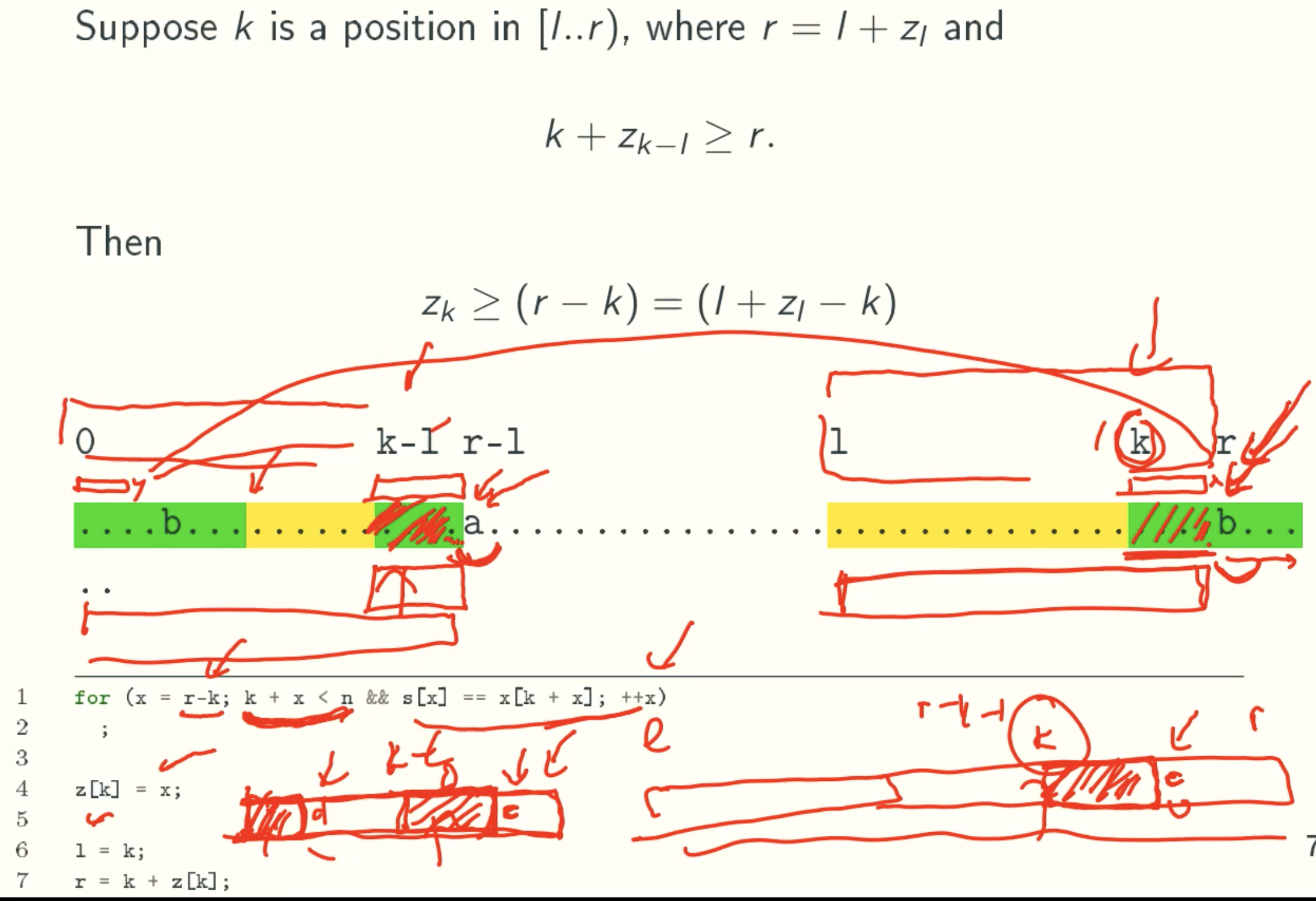
case 3: deducing Zk from a previous z-value

Code

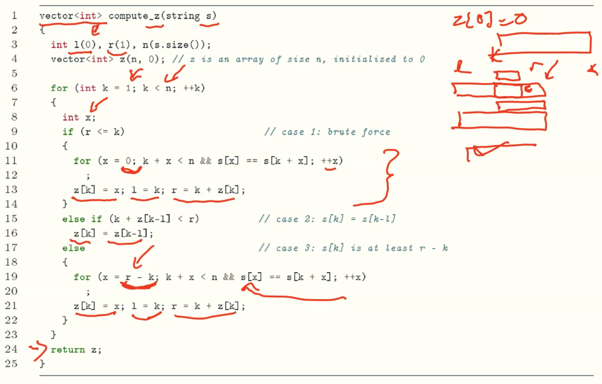
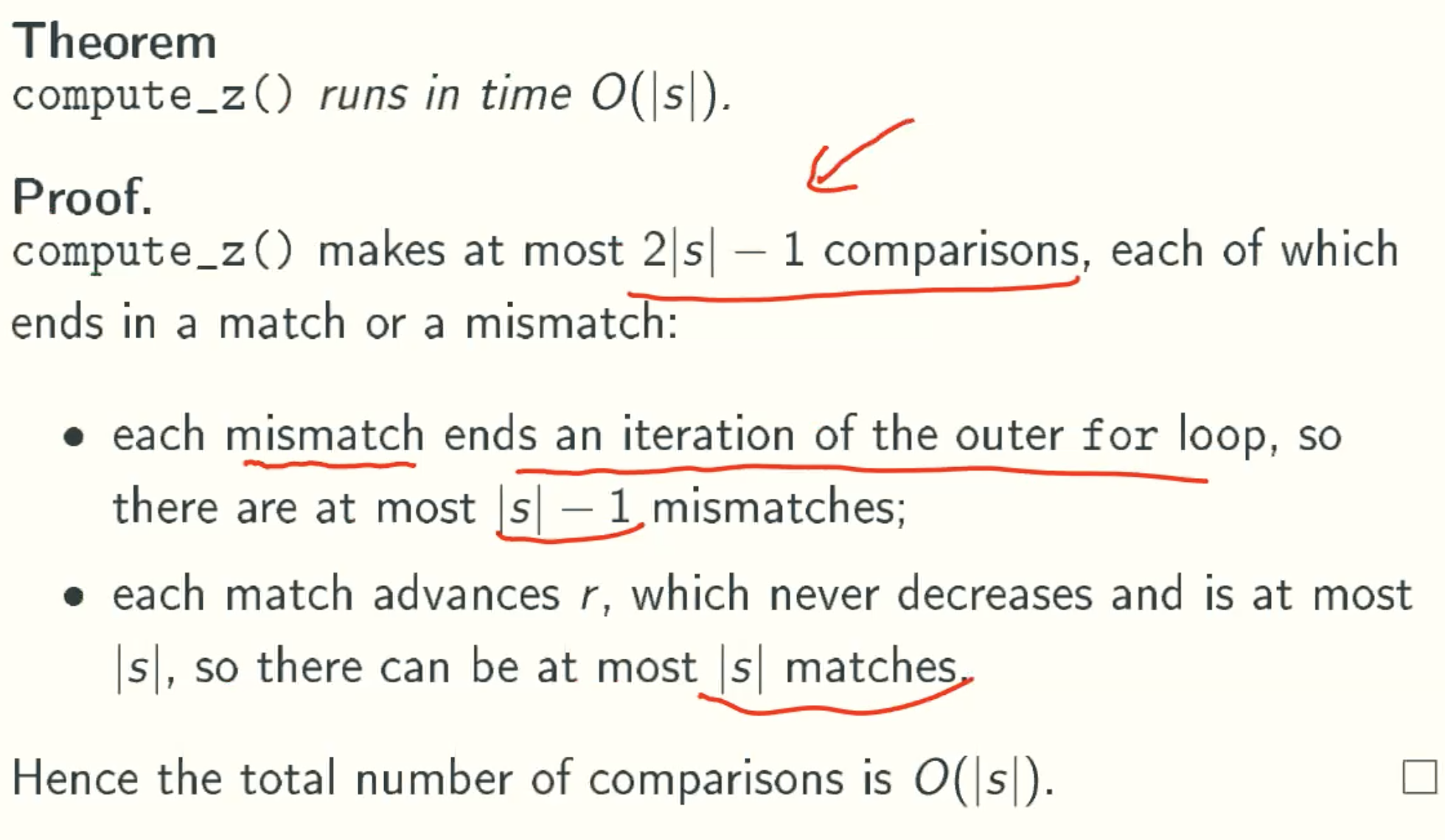
Analysis

Example

A linear-time string matching algorithm

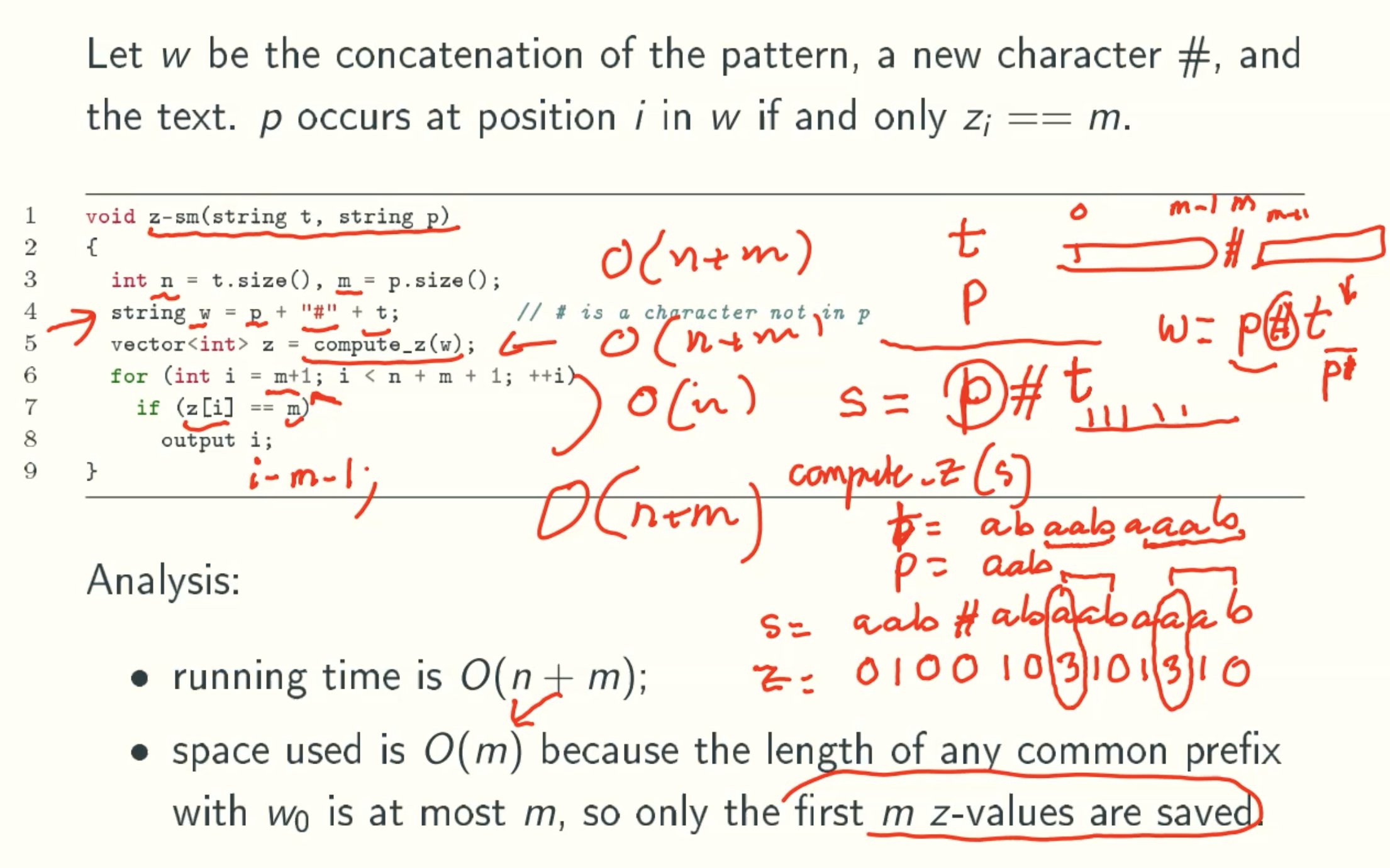
Why space is O(m)

only refer the z[k-l] in algorithm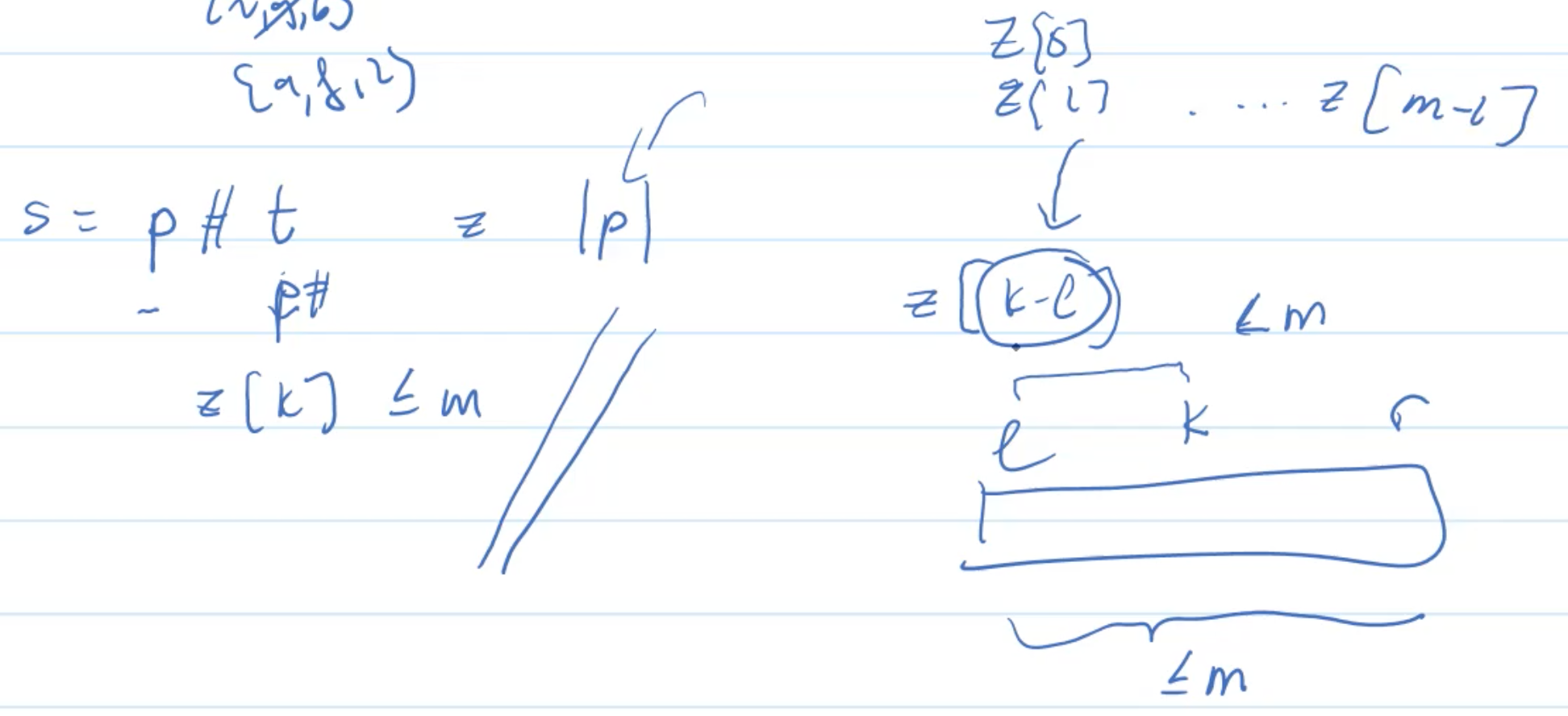

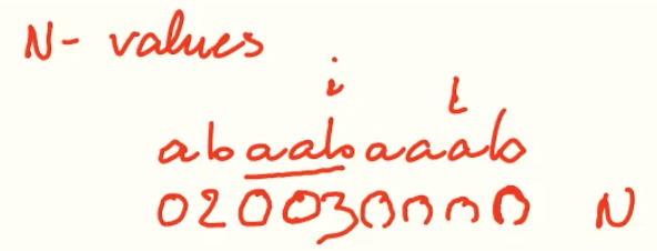
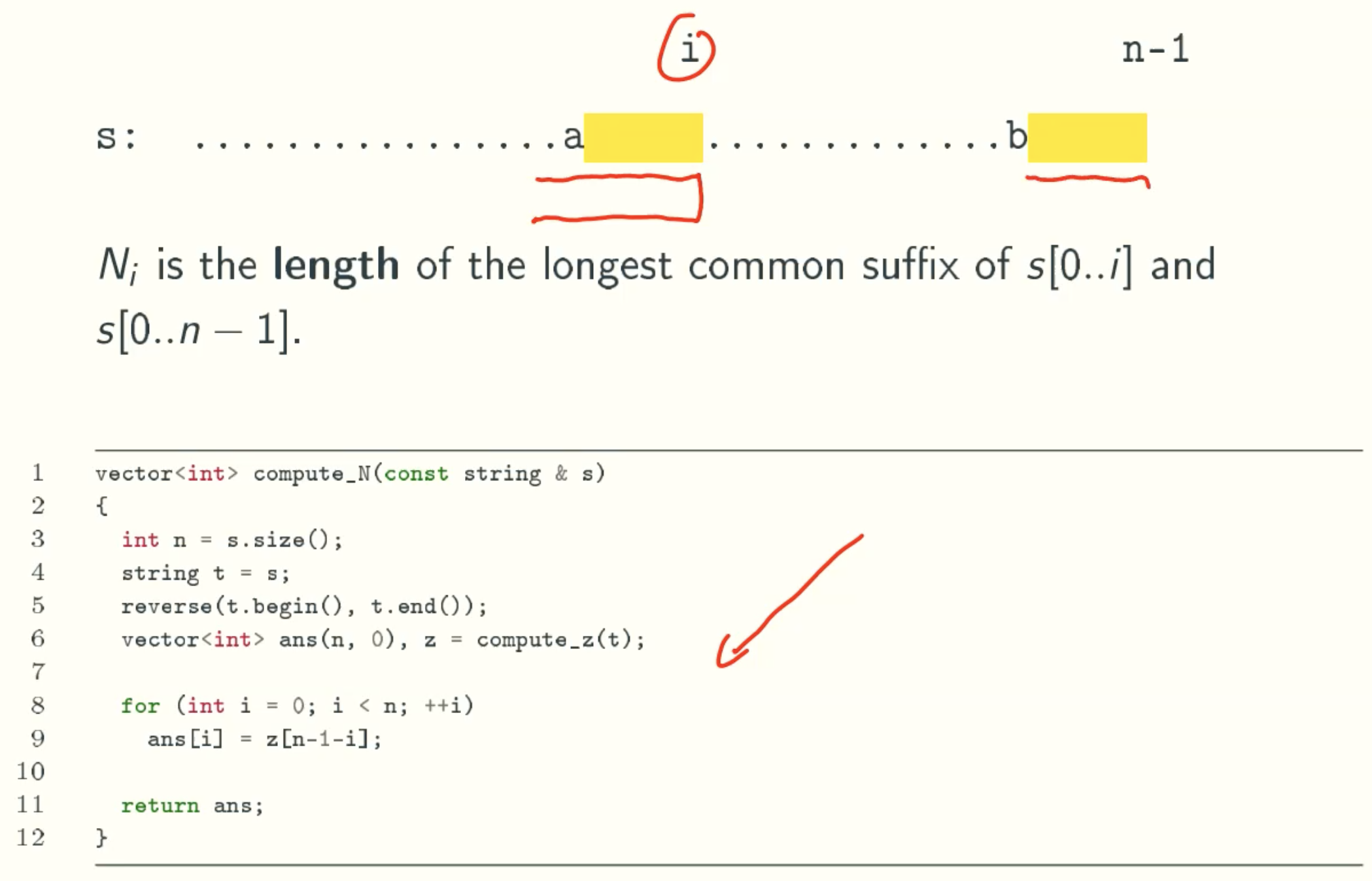
N-value

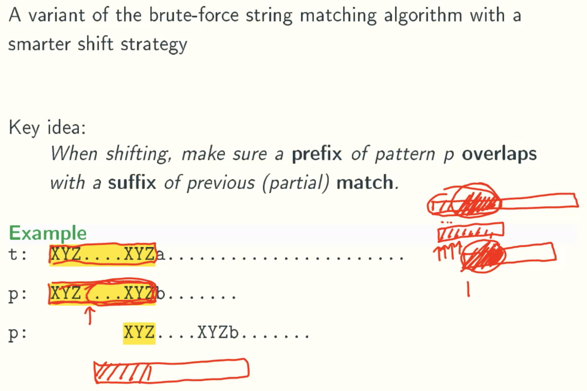
KMP

Overview

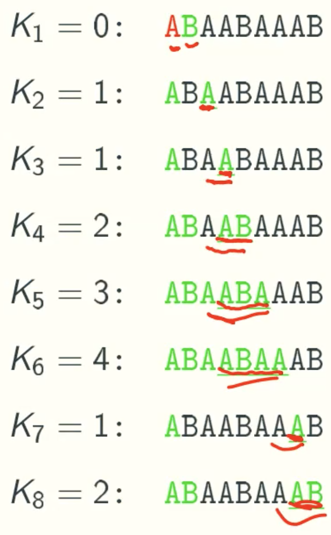
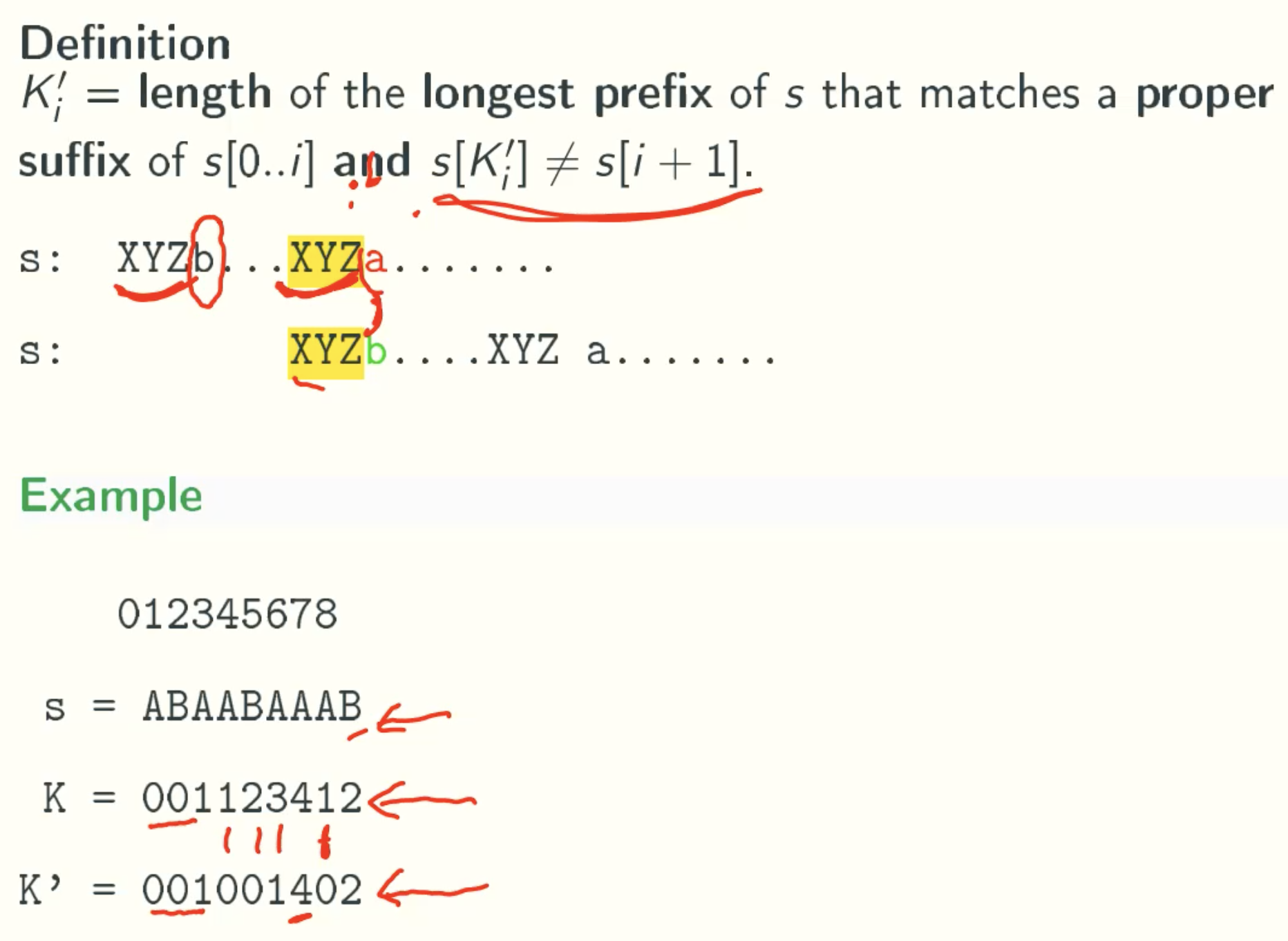
k-values

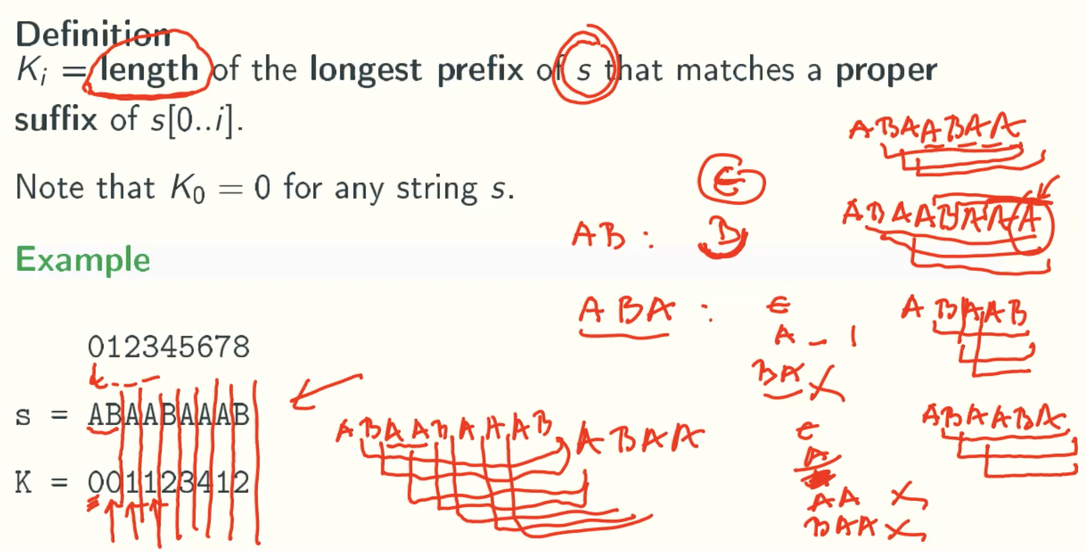
A proper suffix of a string is not equal to the string itself.

In Details

Smarter Shifting

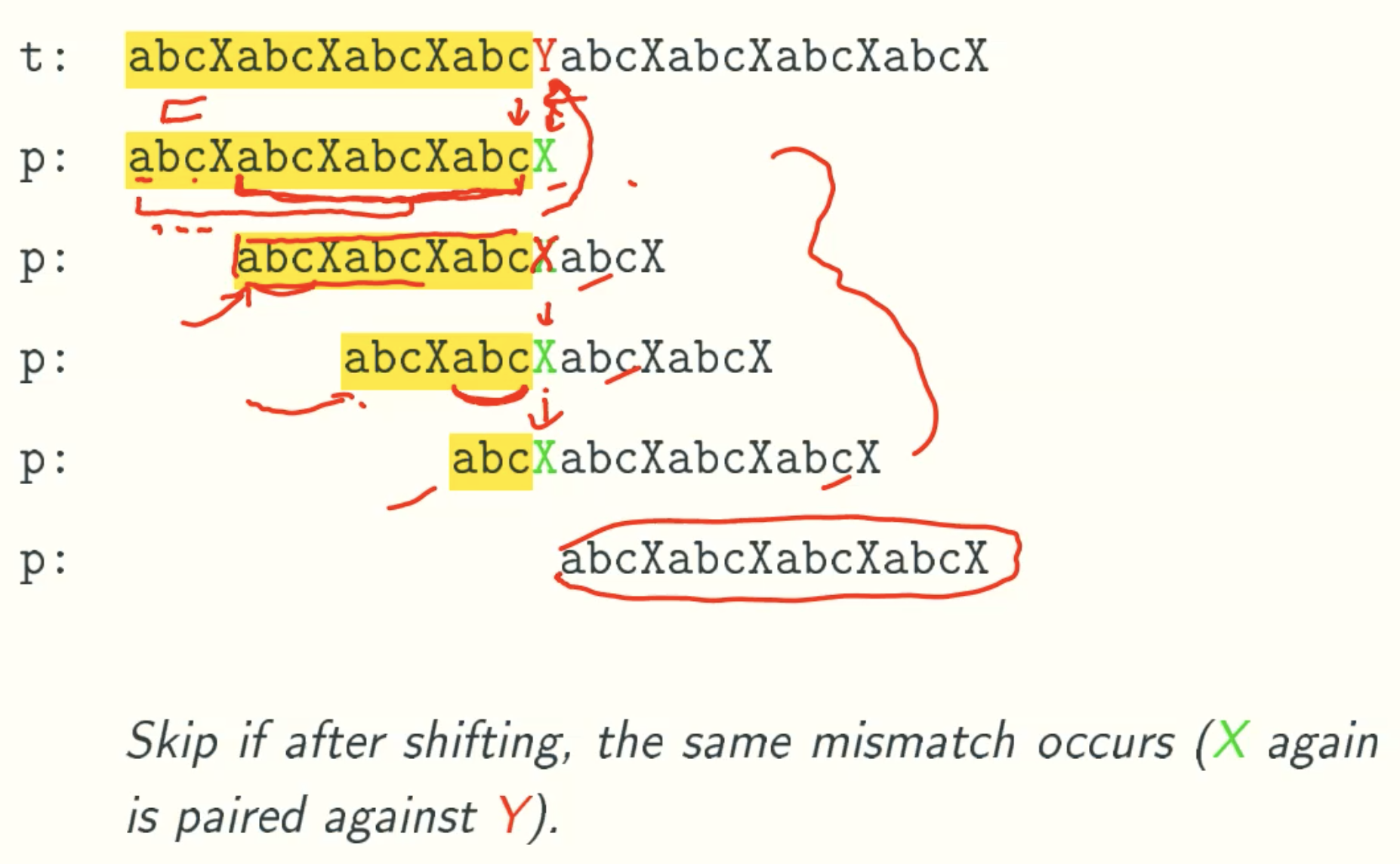
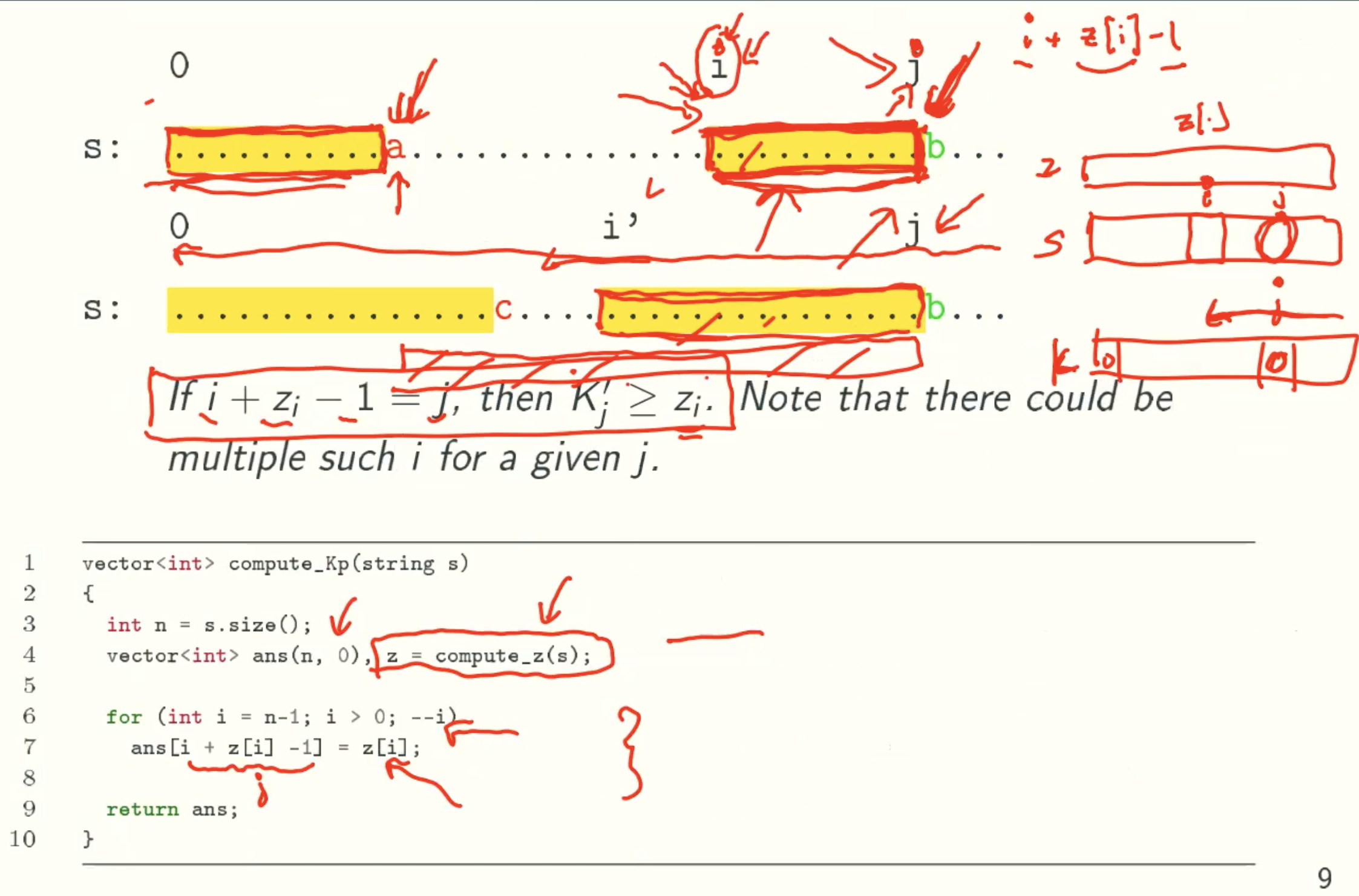
k’-values

In Details

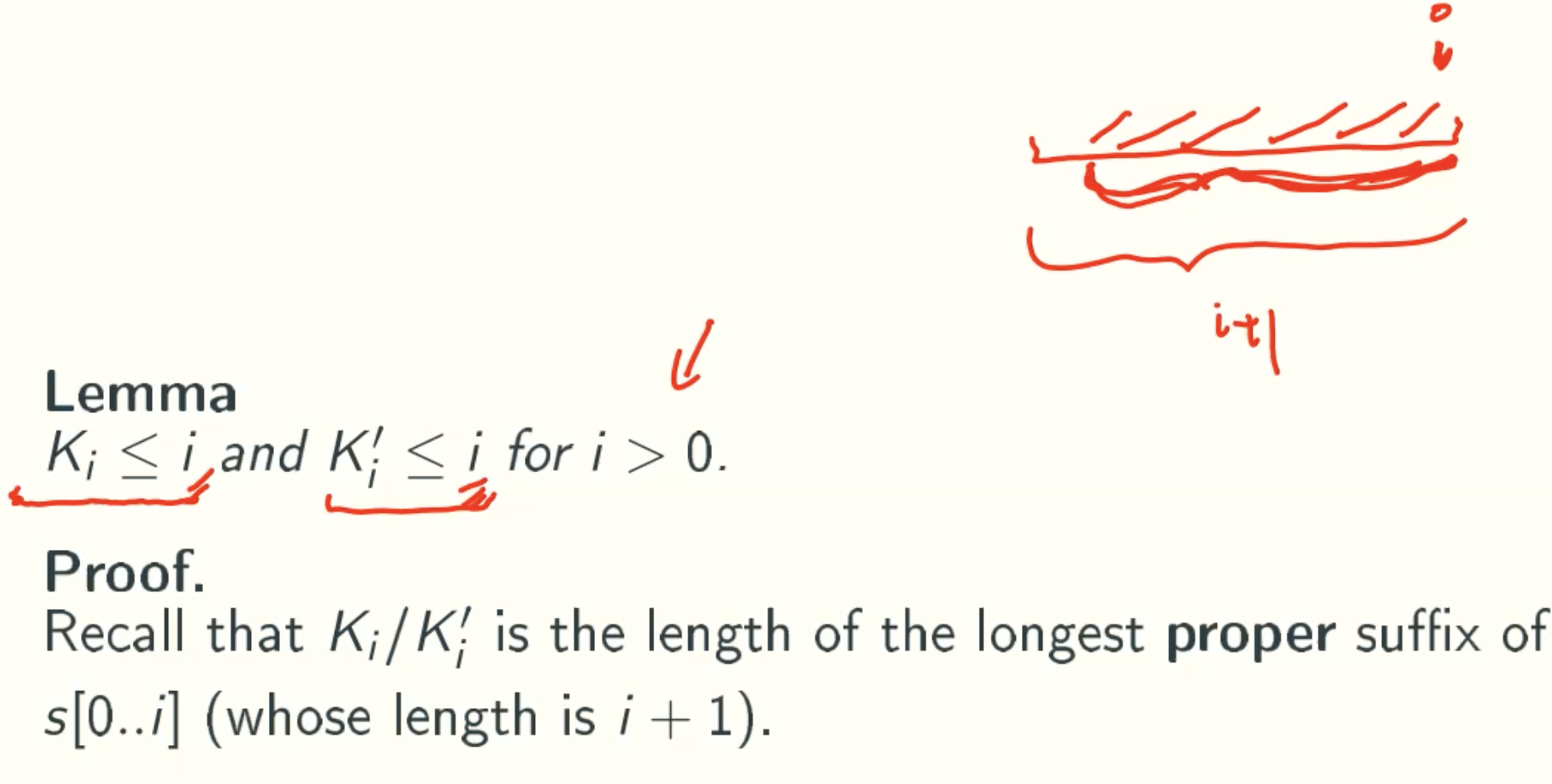
Property of K/K’-Values

Computing K/K’-values In Linear Time

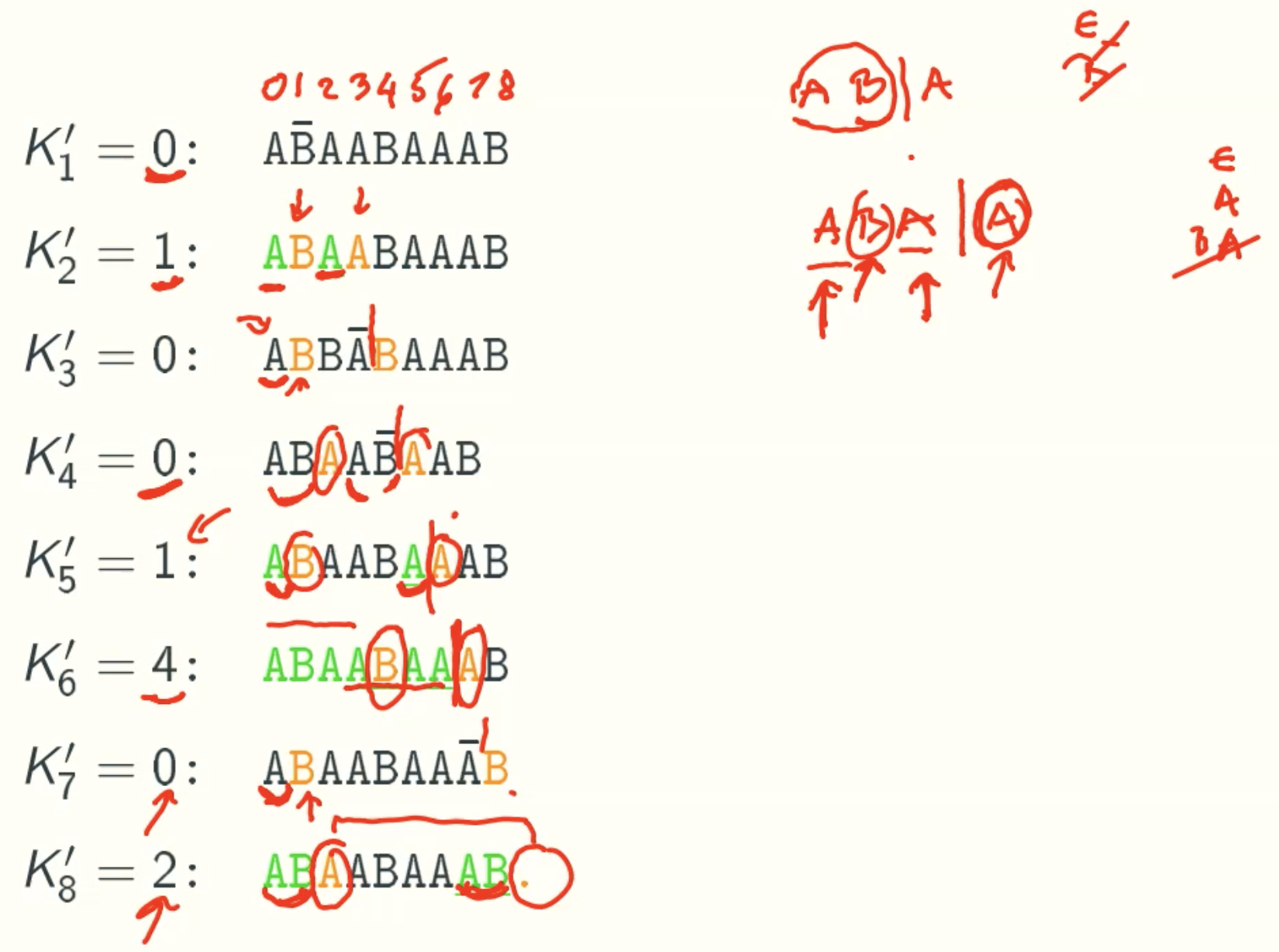
K’-Values

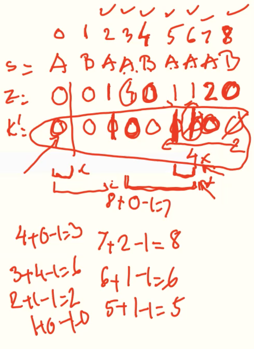
Example

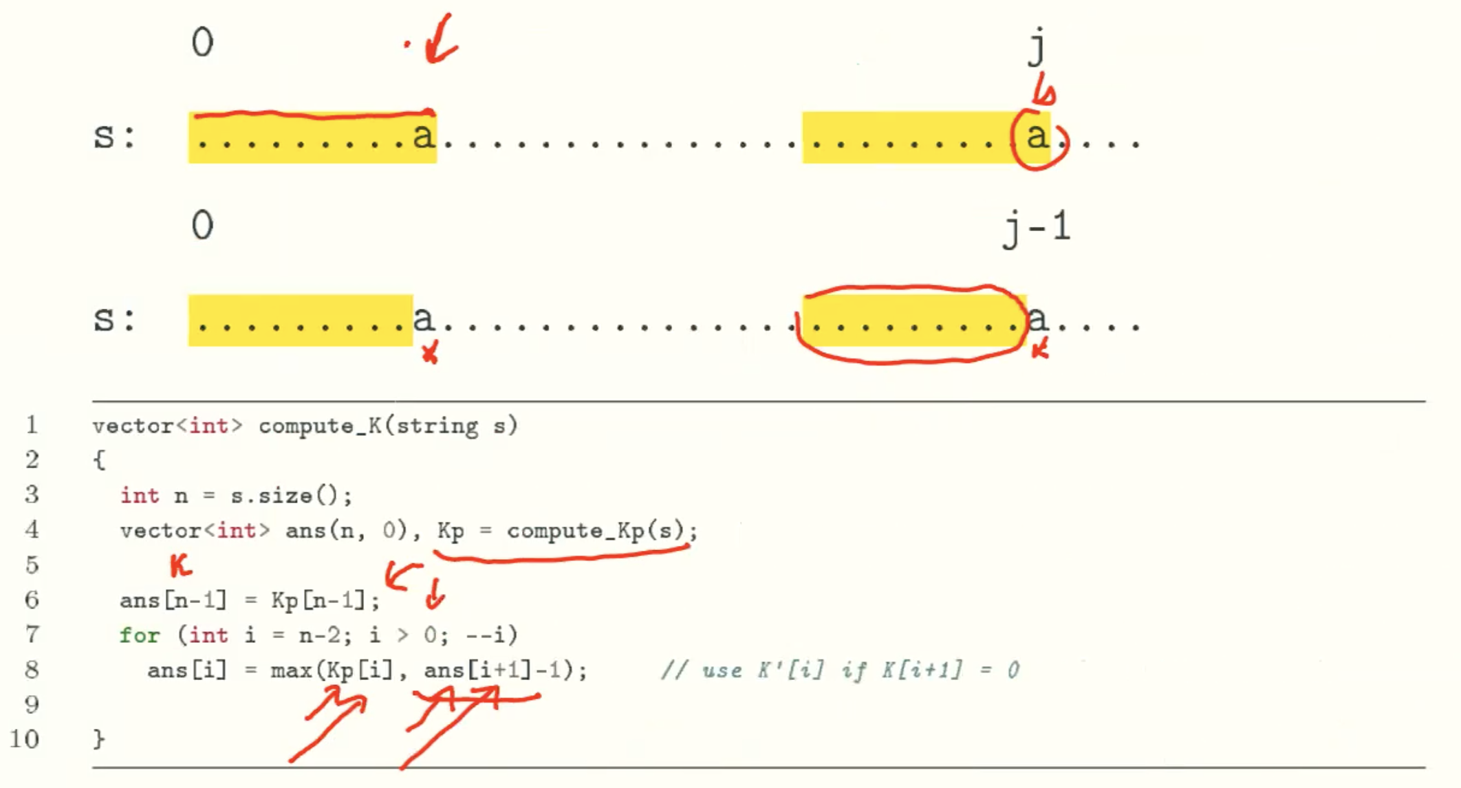
K-Values

A linear-time string matching algorithm-KMP

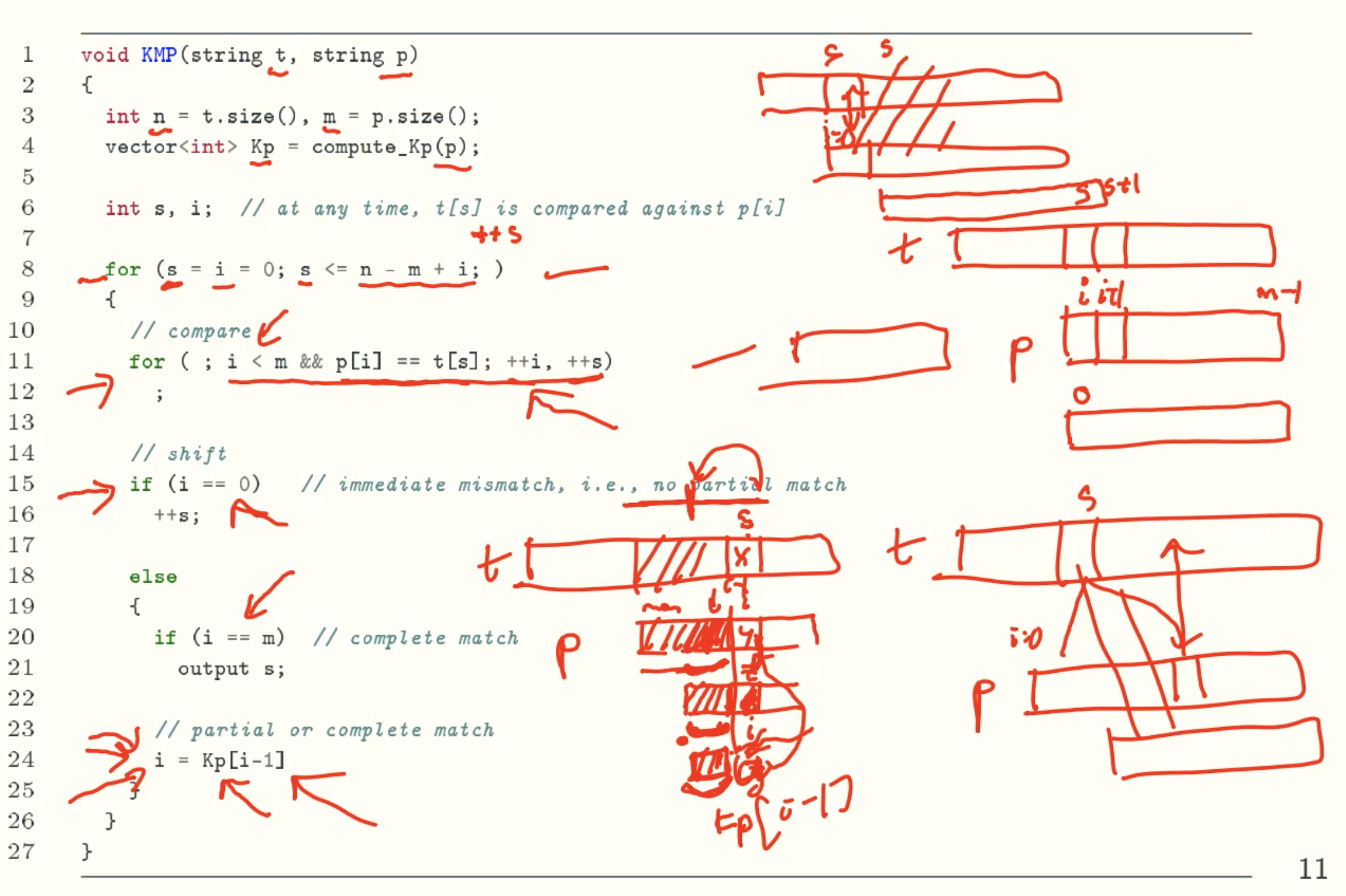
Example

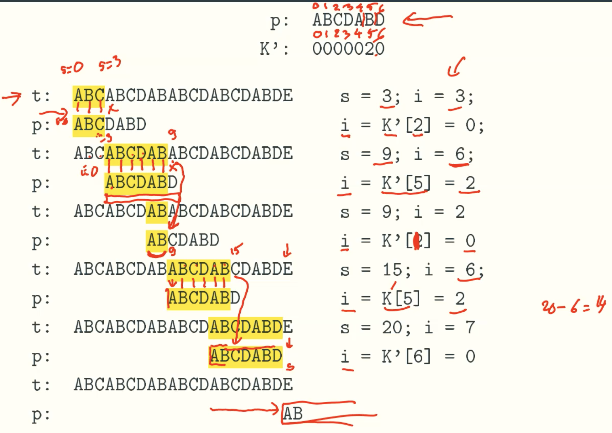
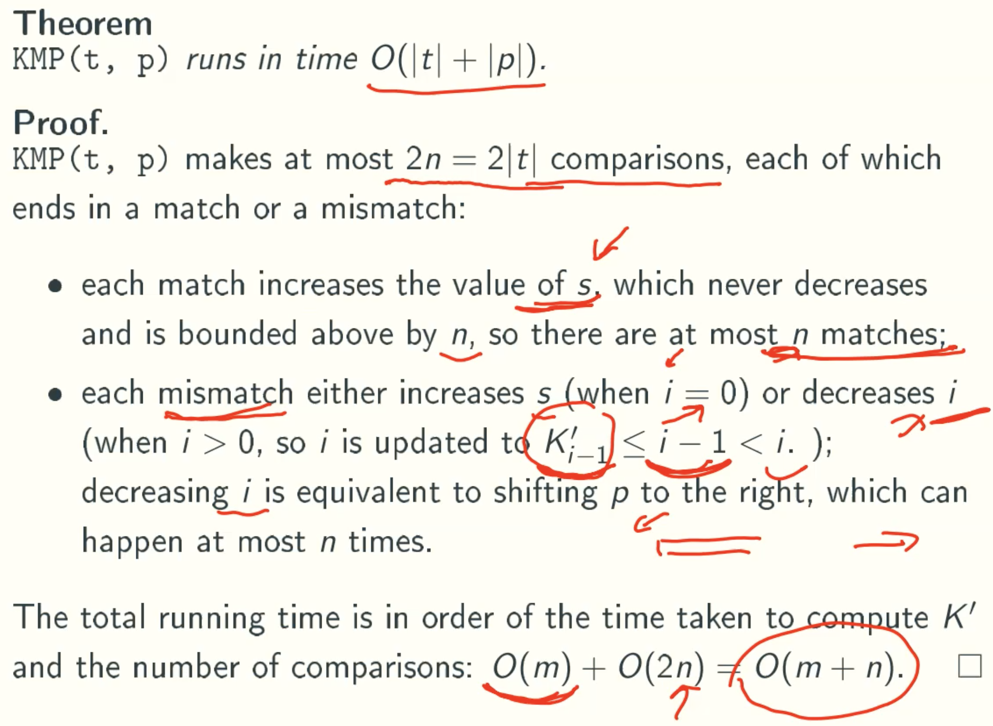
Analysis

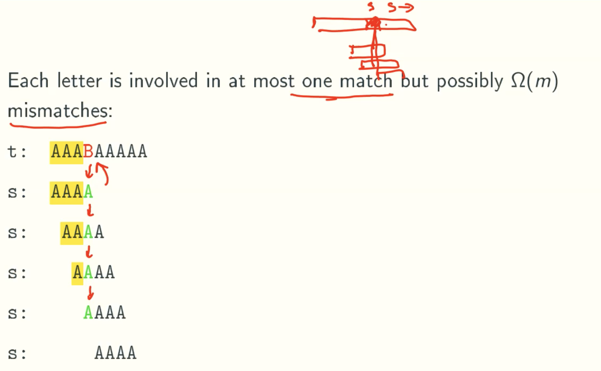
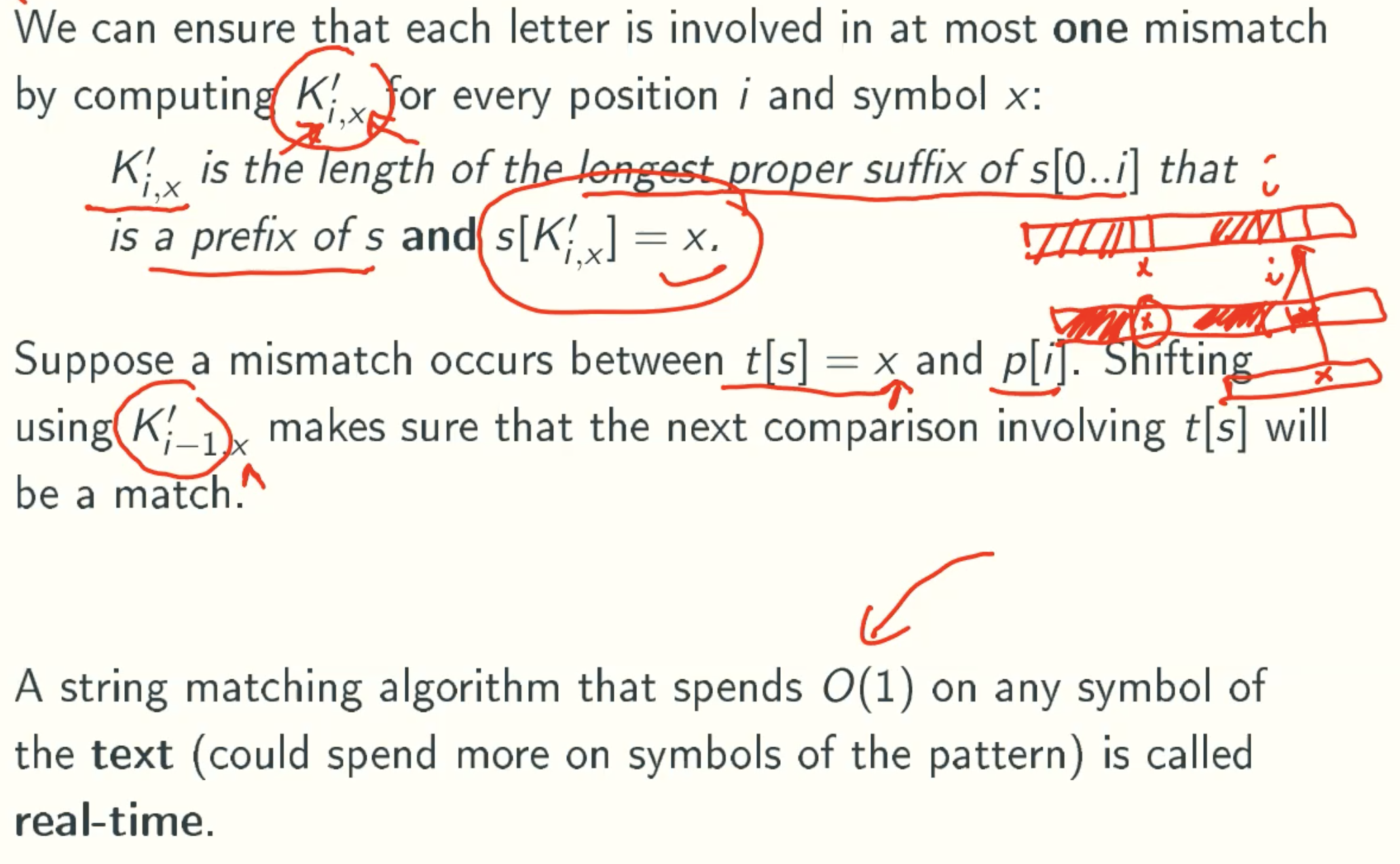
Real-time Version of KMP

K’_i,x

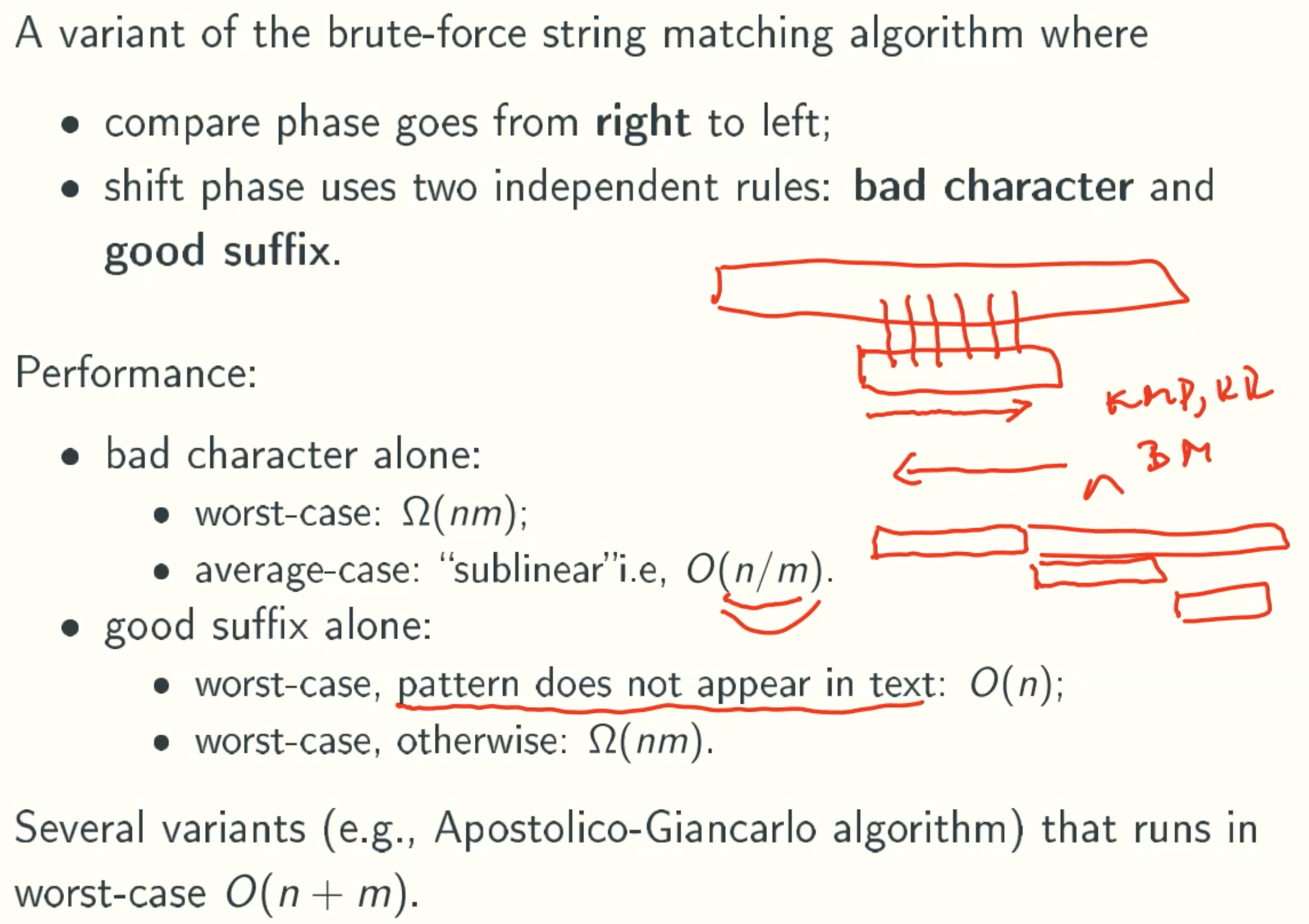
BOYER-MOORE(BM) Algorithm

Overview

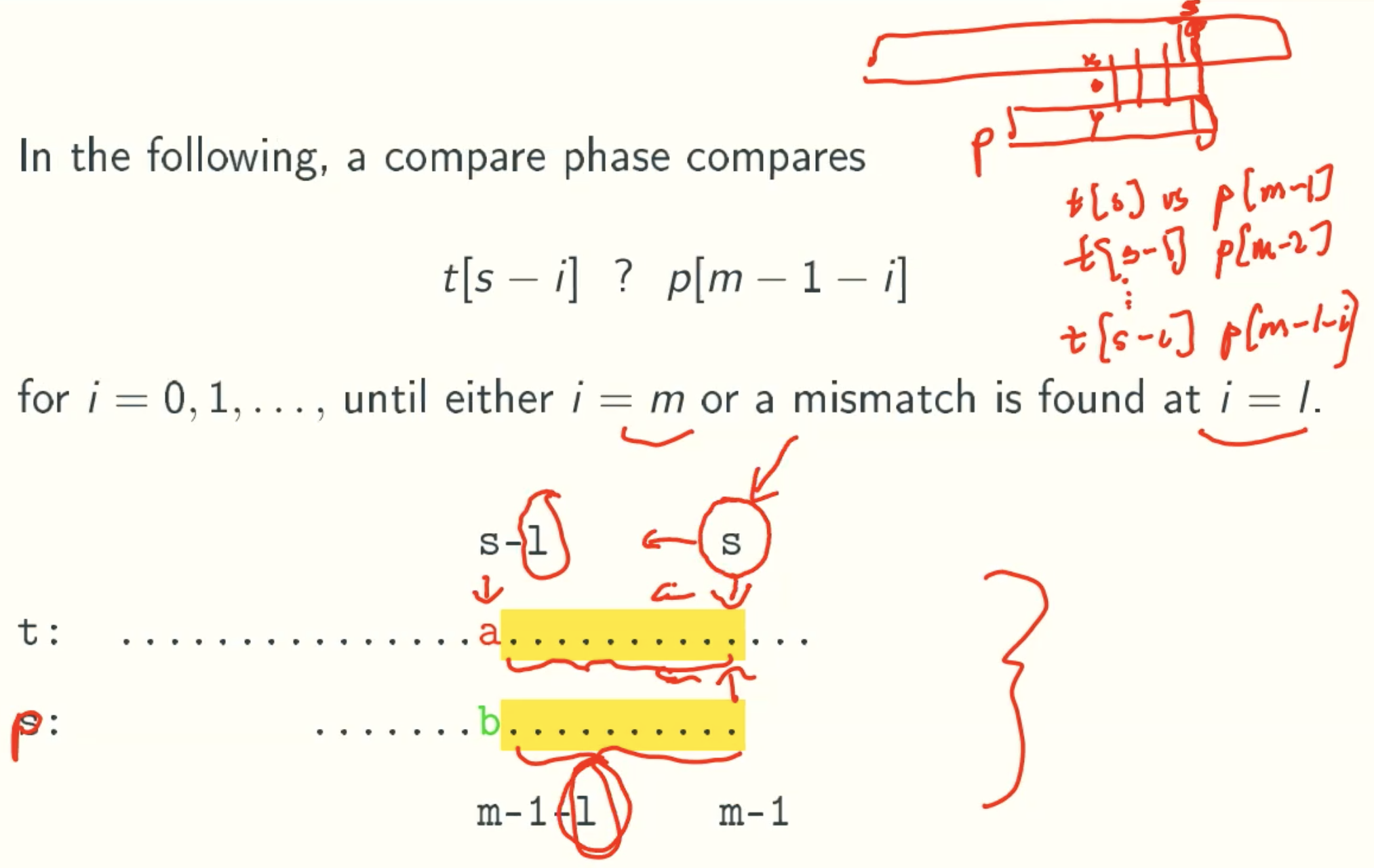
Notation

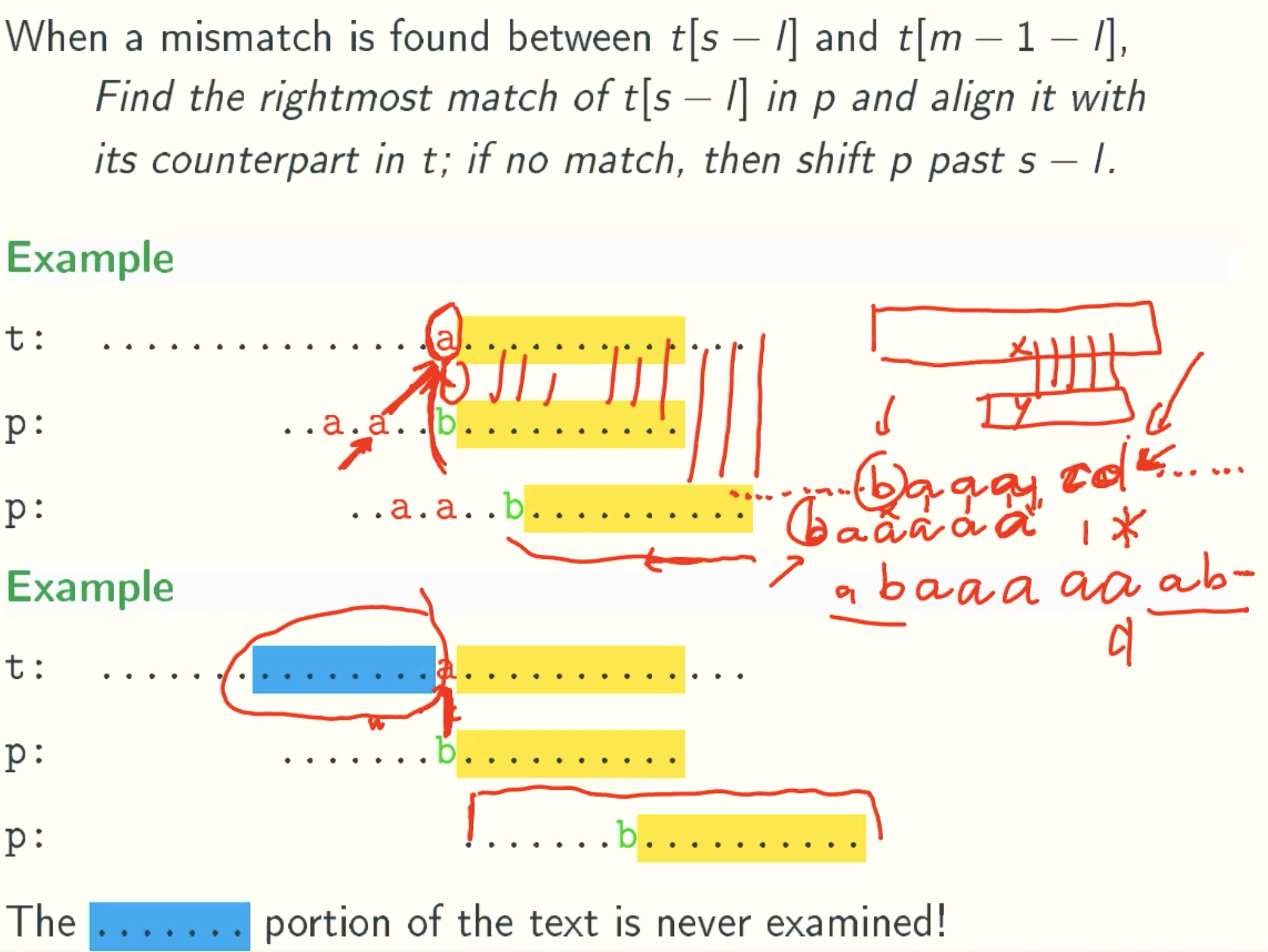
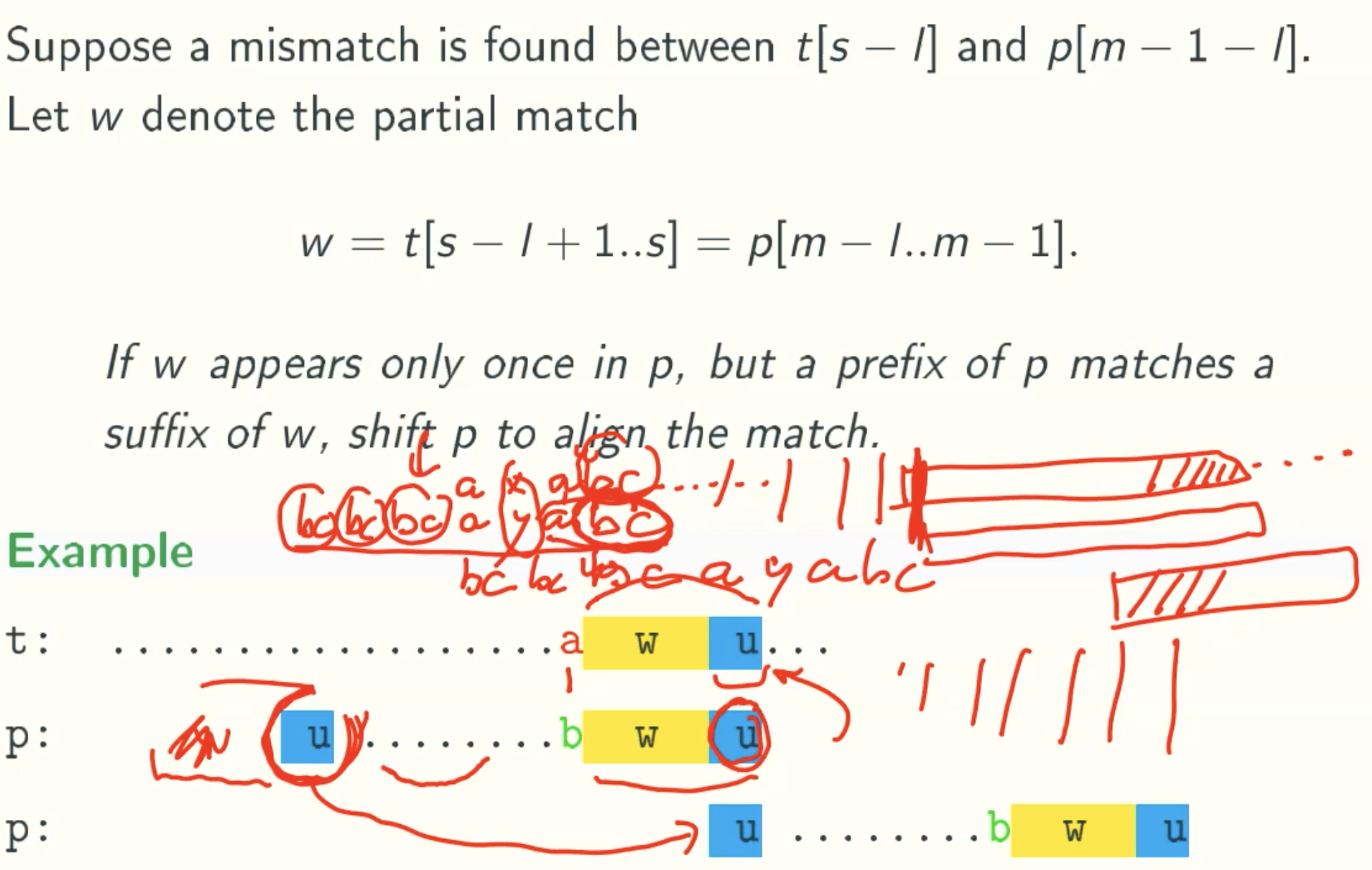
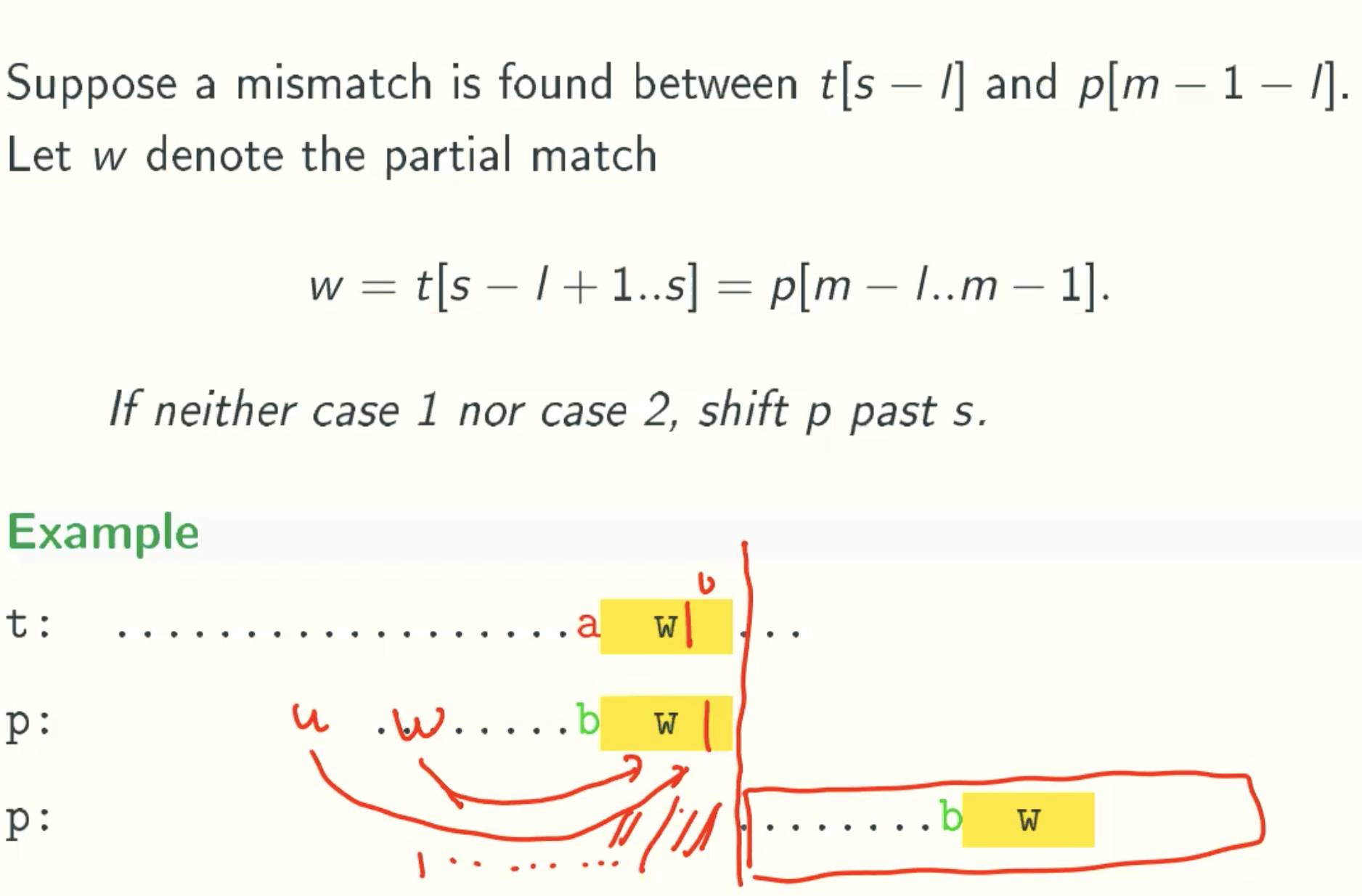
Bad Character Rule

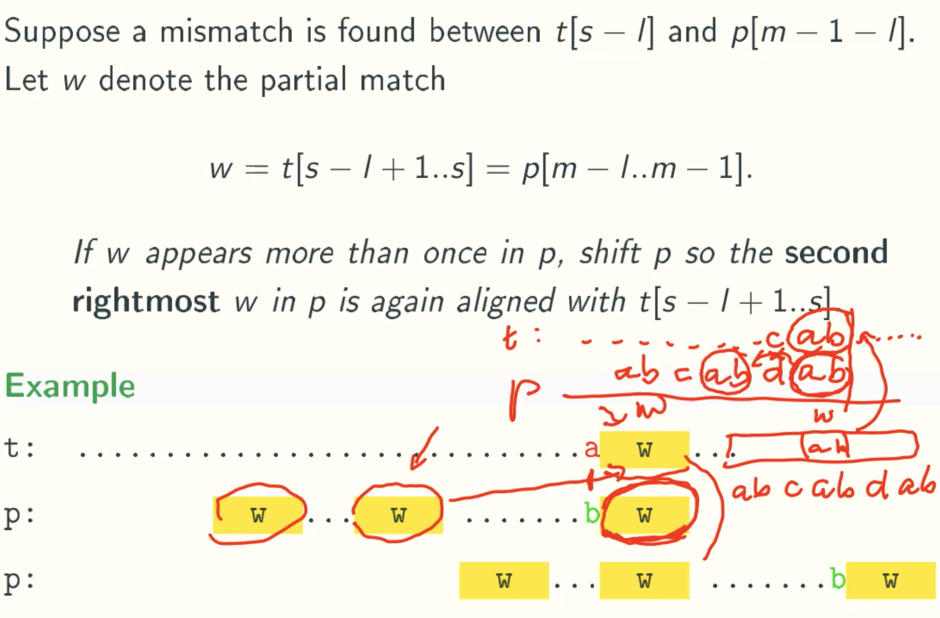
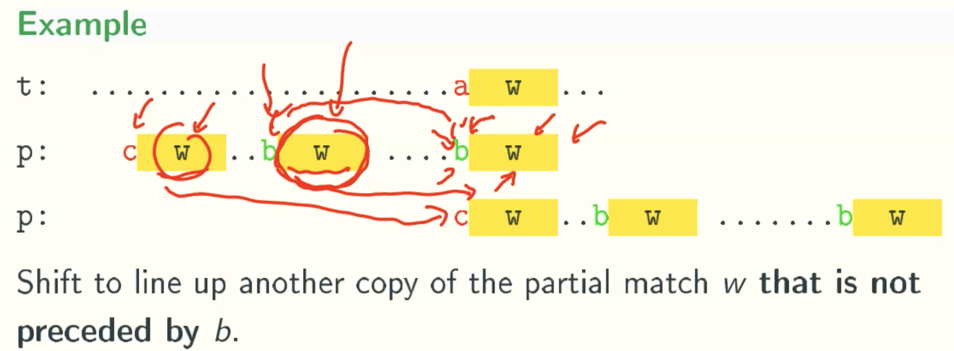
Good Suffix Rule

Rule 1

Rule 2

Rule 3

BOYER-MOORE(BM): Complete Shifting Rule

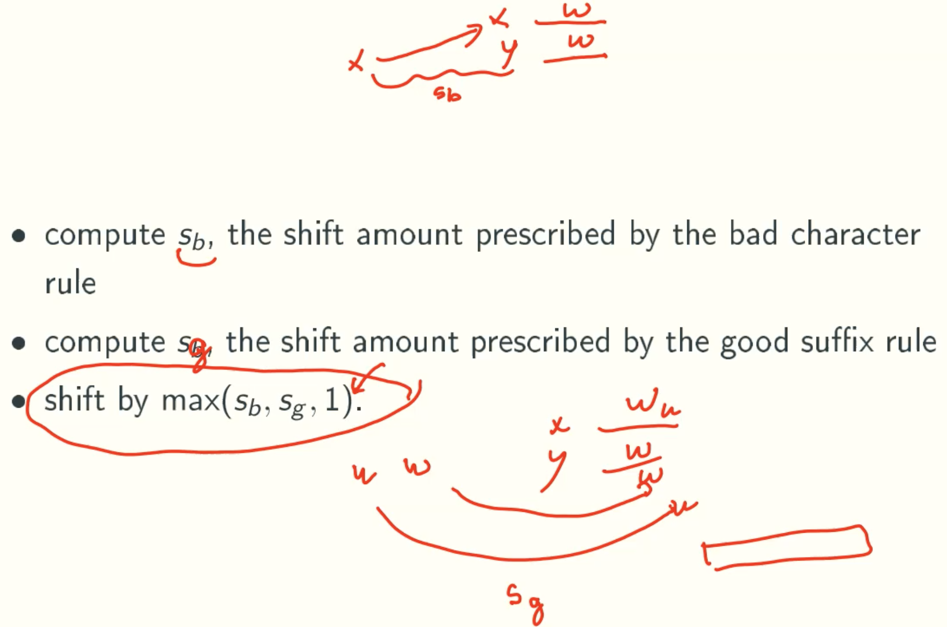
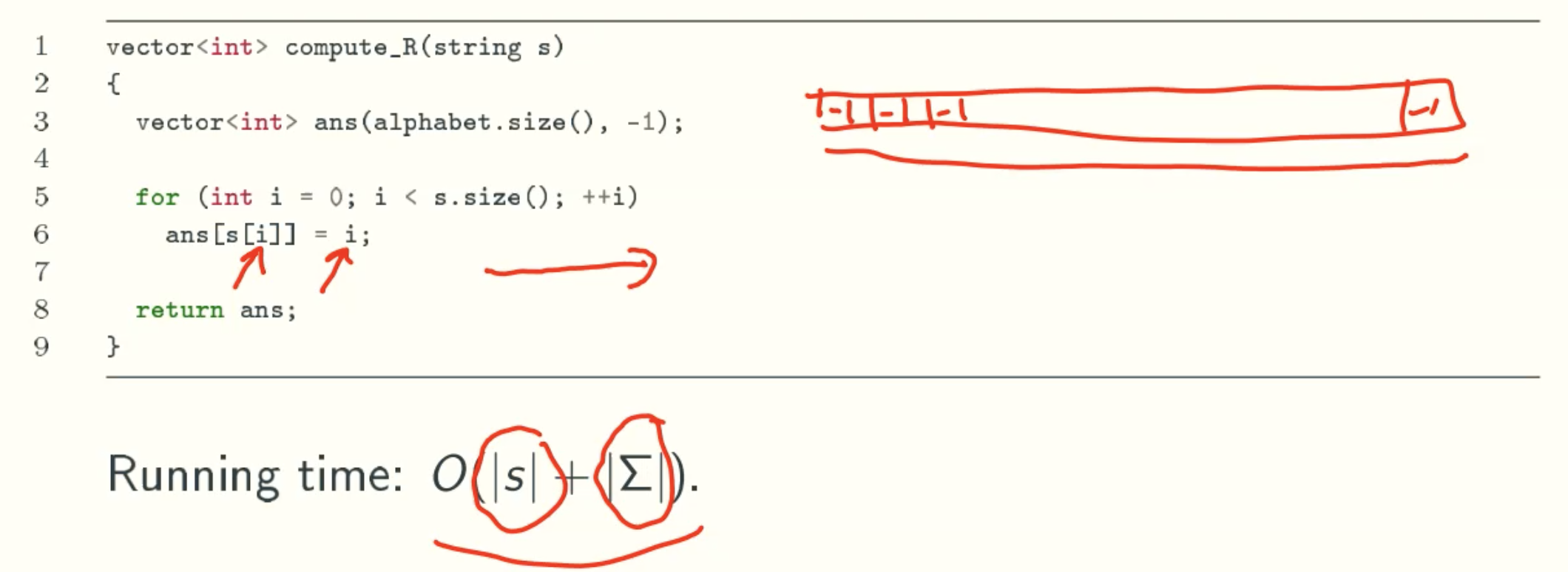
Implementation Of Bad Character Rule

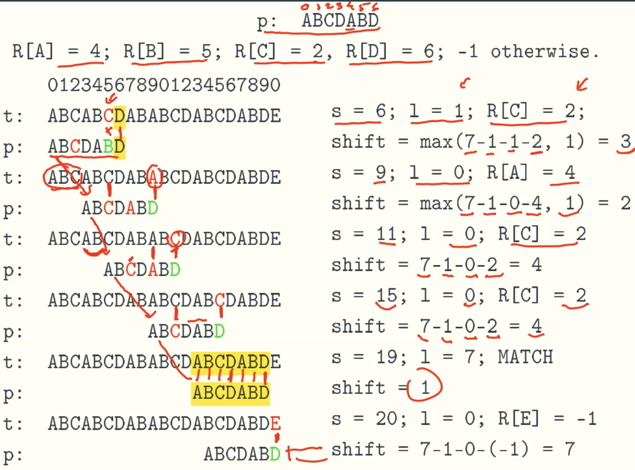
R[c]: rightmost position of c

Code Implementation

S_b: Shift amount of the bad character rule

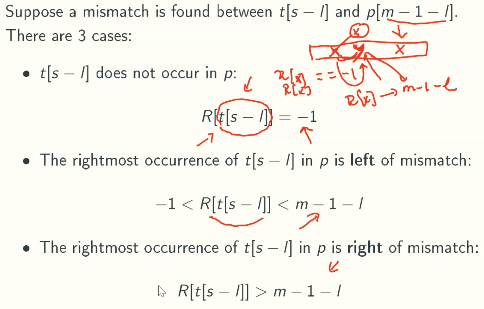
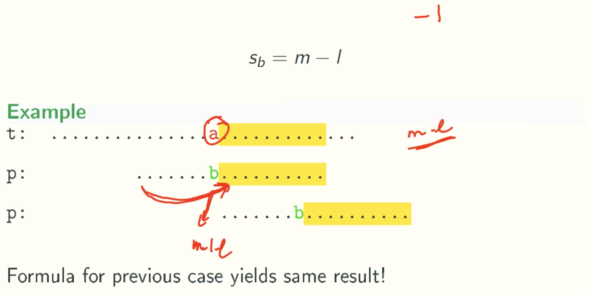
Case 1

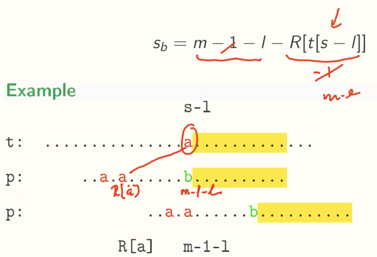
Case 2

Case 3 - Back To Brute Force

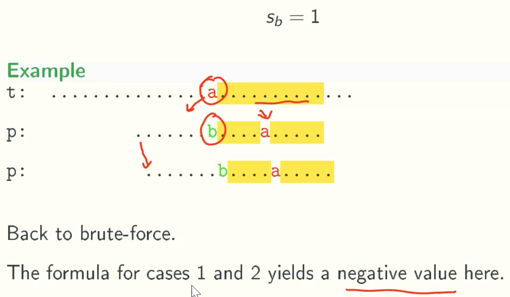
General Formula

S_b = max(m-1-l-R[t[s-l]], 1)

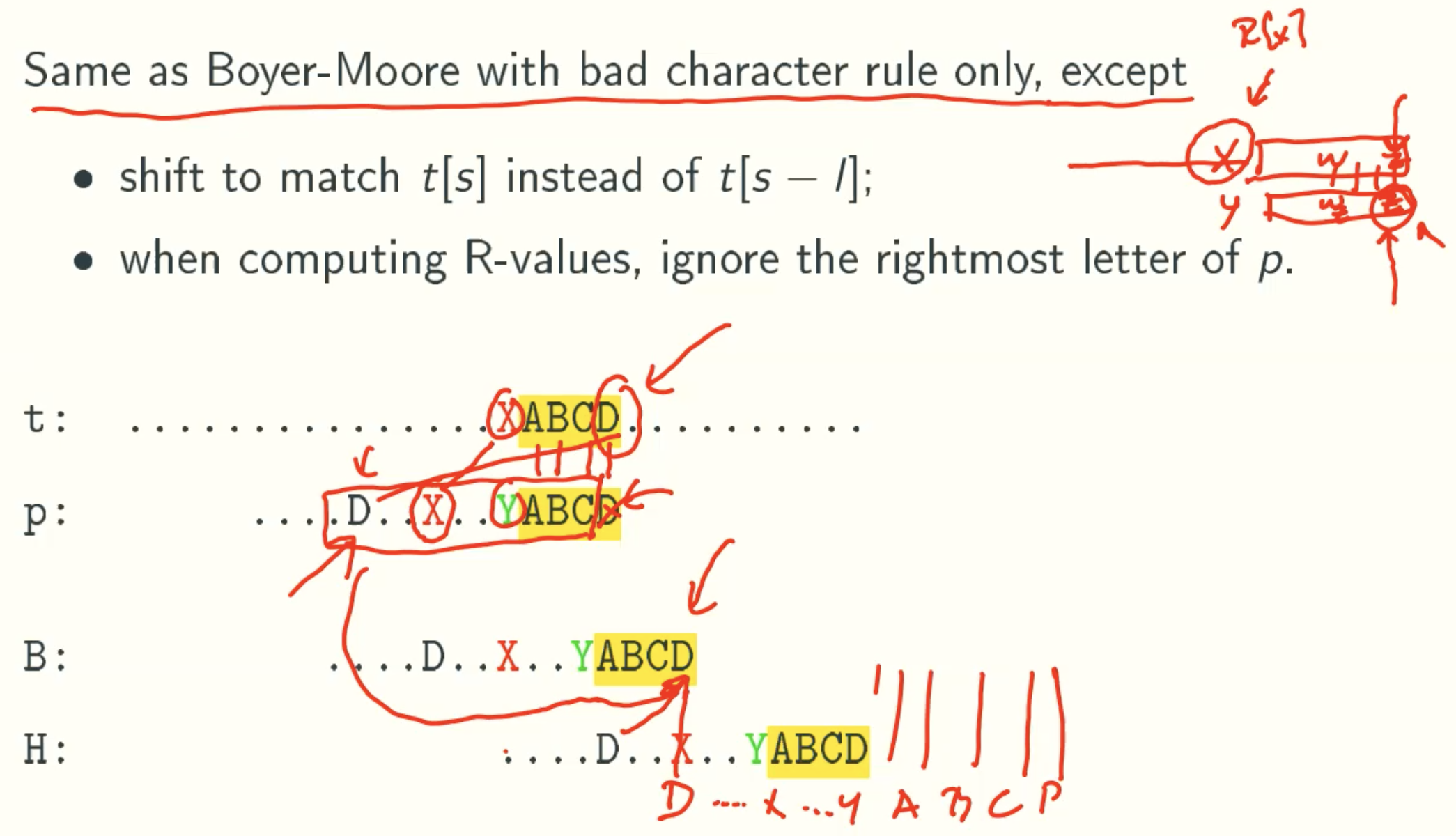
BOYER-MOORE(BM) Implementation: bad character rule only

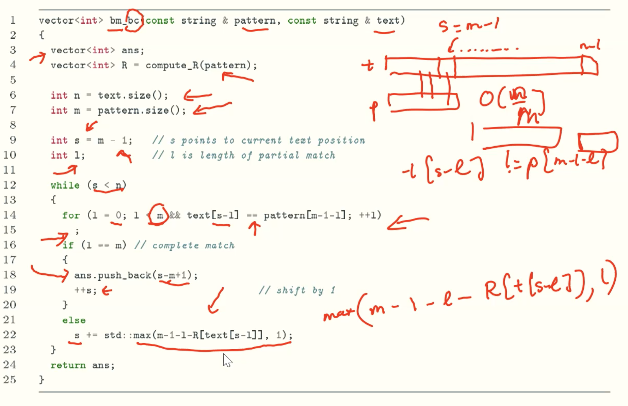
Example

Horspool algorithm

Implementation Of Good Suffix Rule

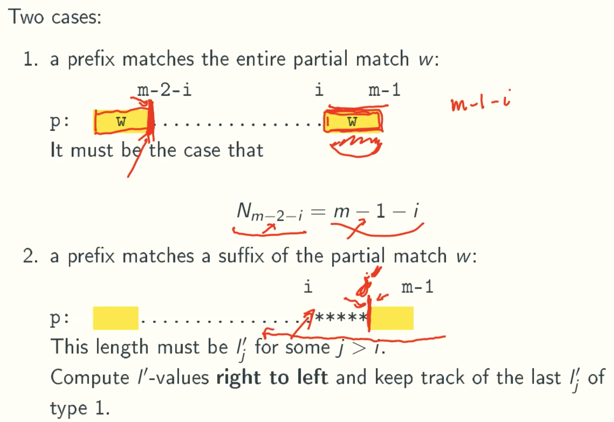
Case 1

N Value

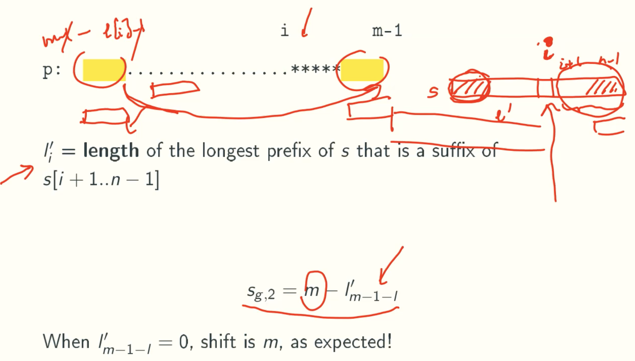
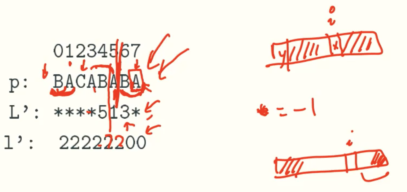
L’ Value

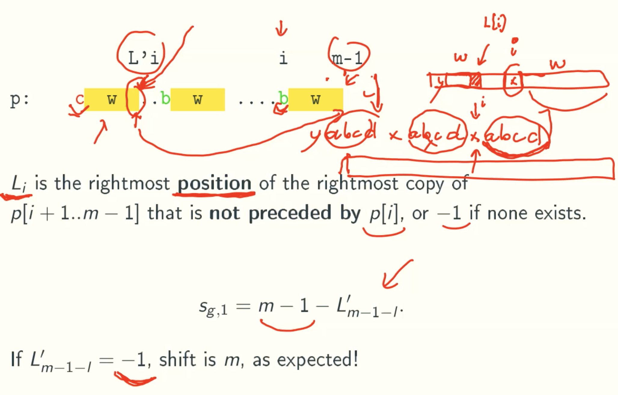
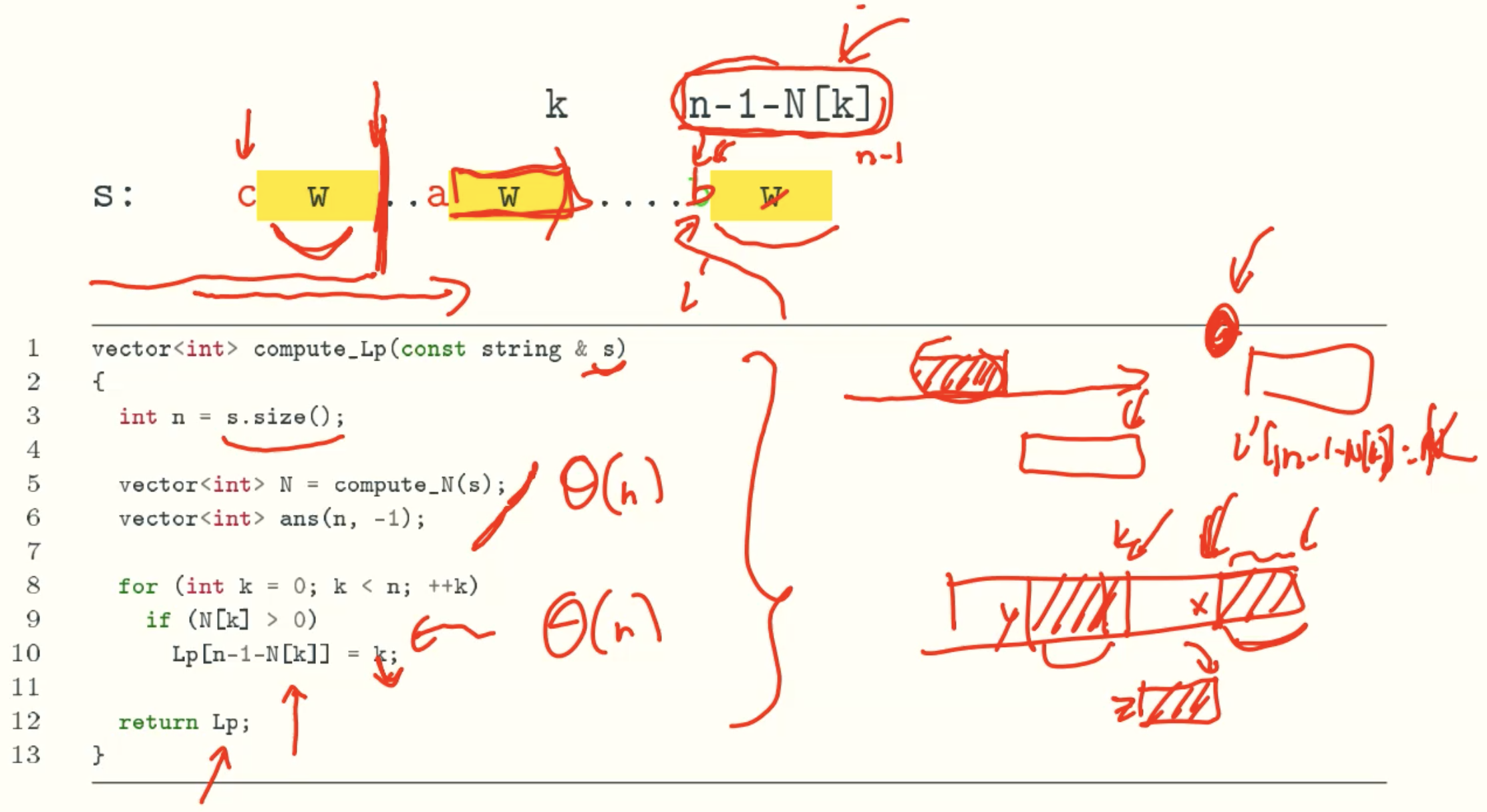
Case 2

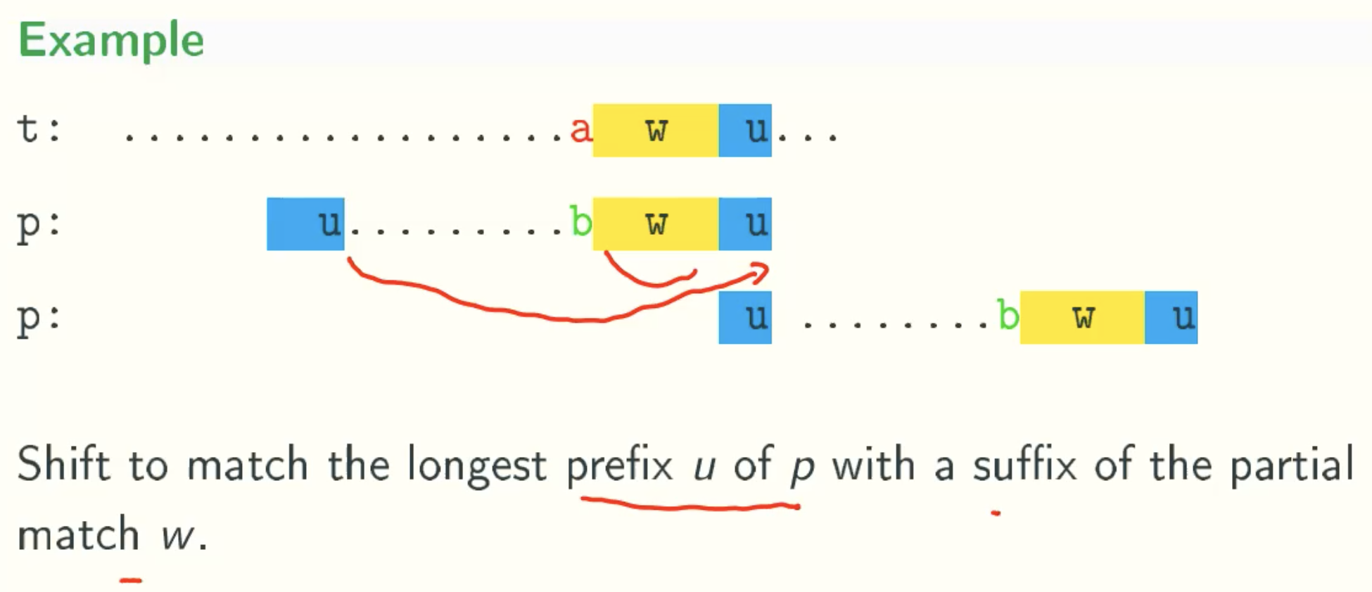
I Value

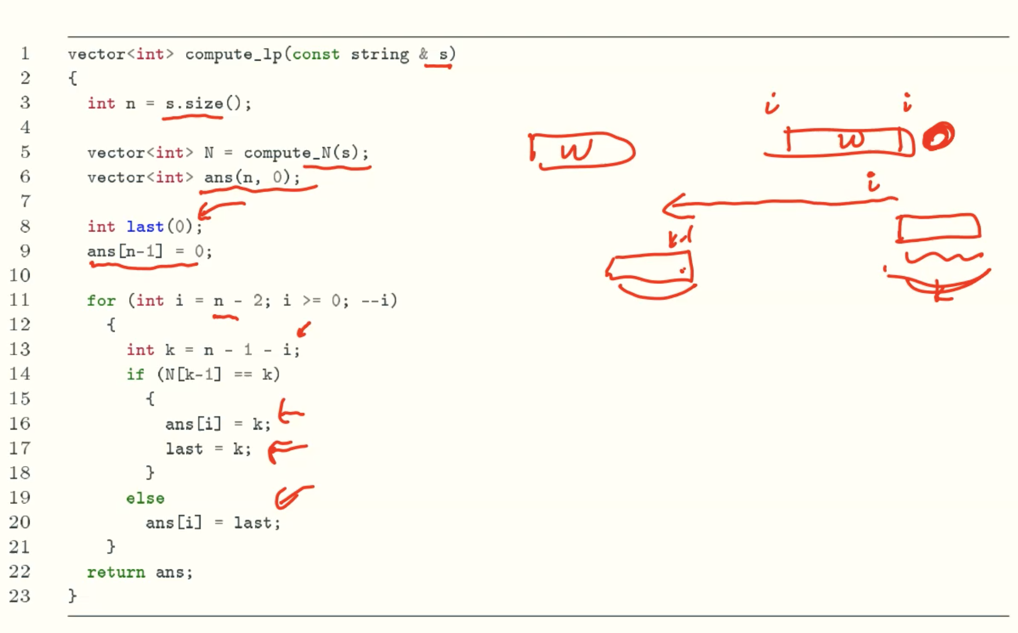
Computing

Code

Case 3

Neither case 1 or 2 applies: shift by m

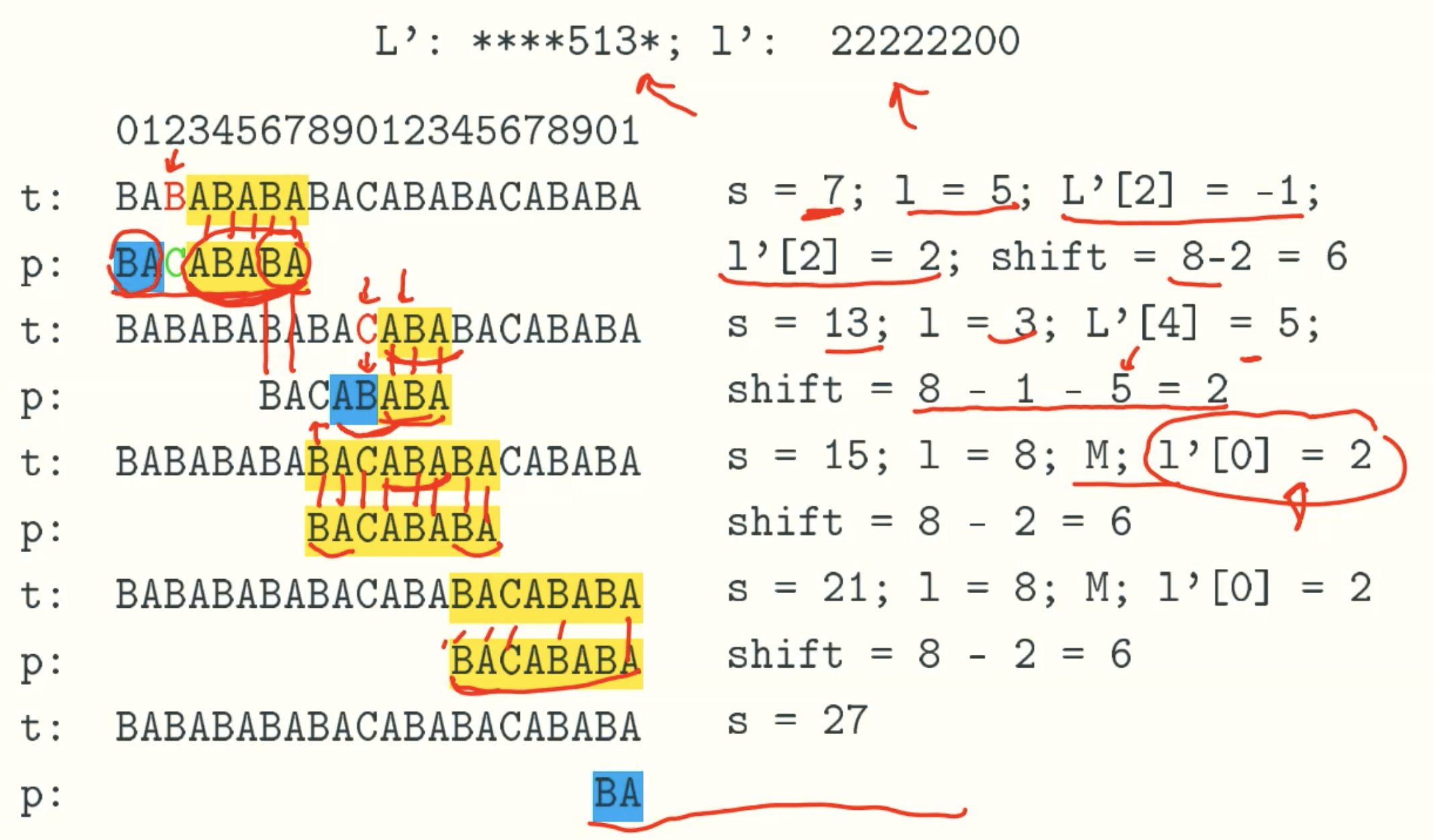
Implementation Of BOYER-MOORE(BM) Algorithm

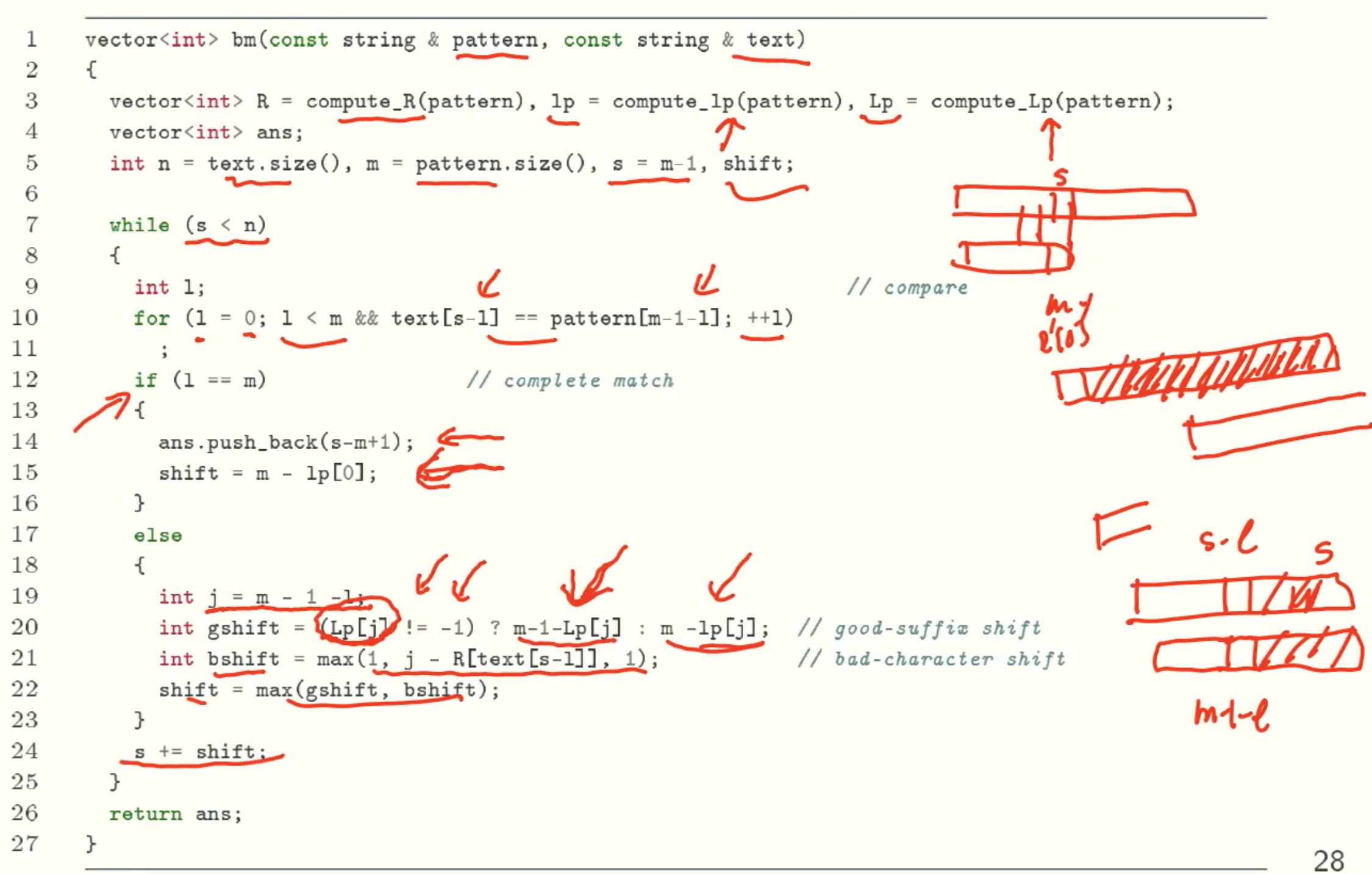
Example

Suffix Trees

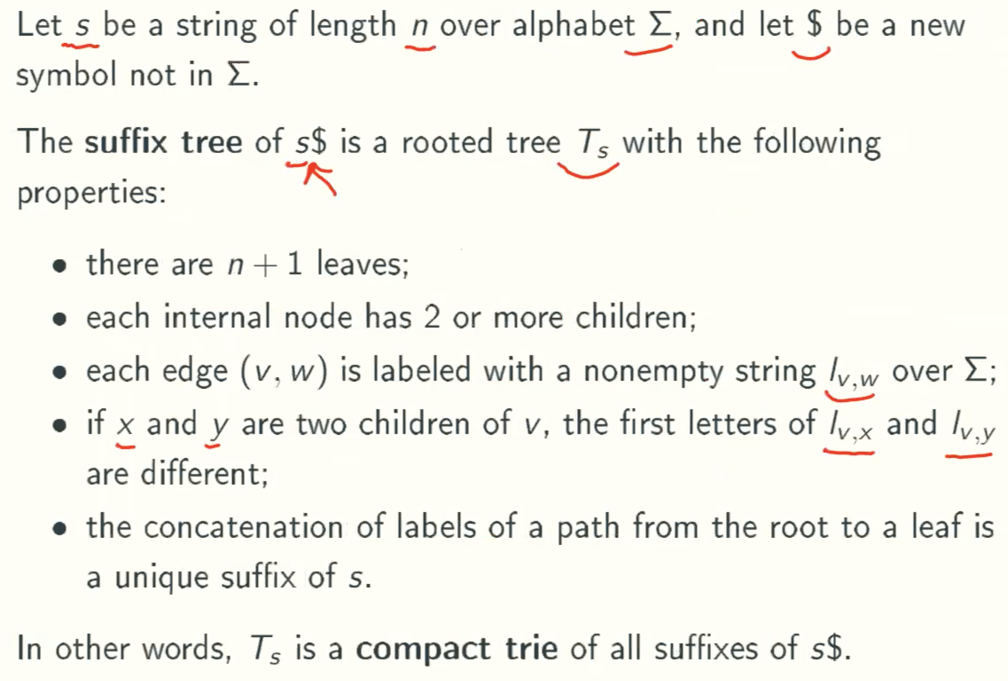
Definition

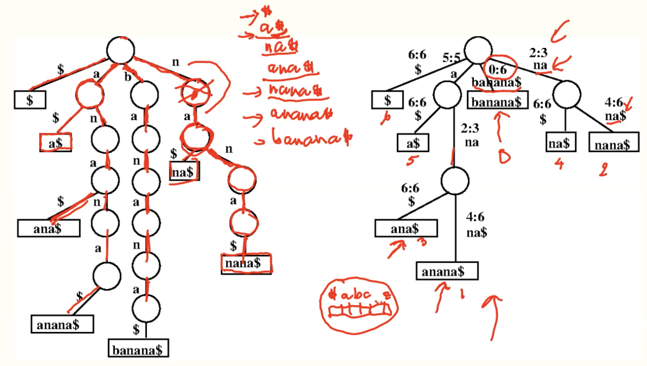
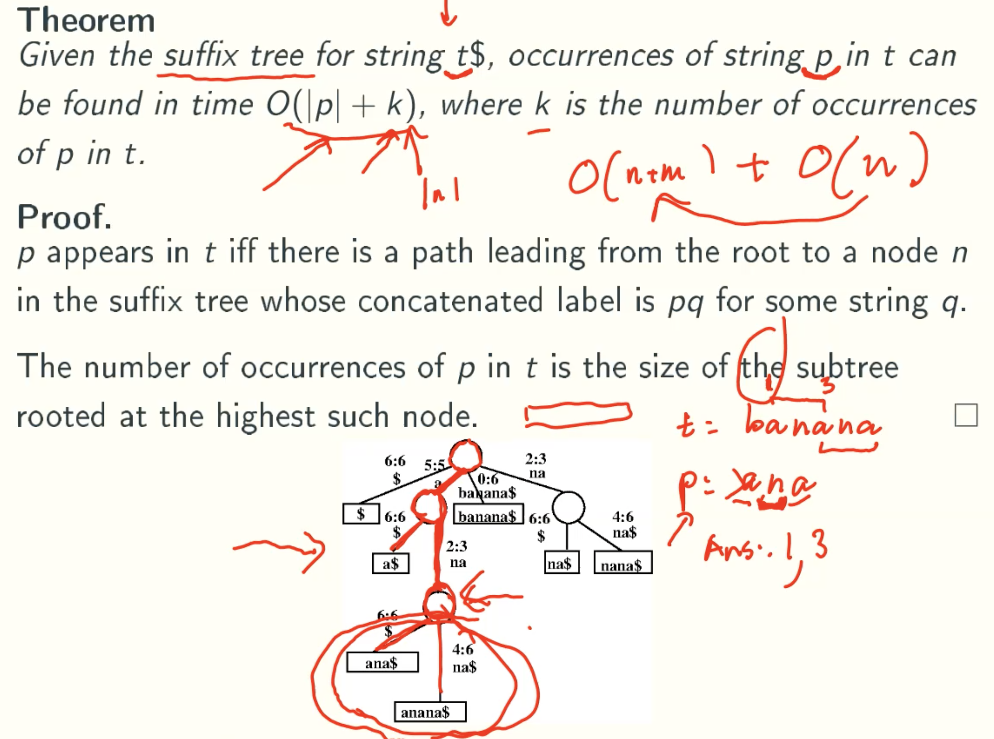
Example: banana

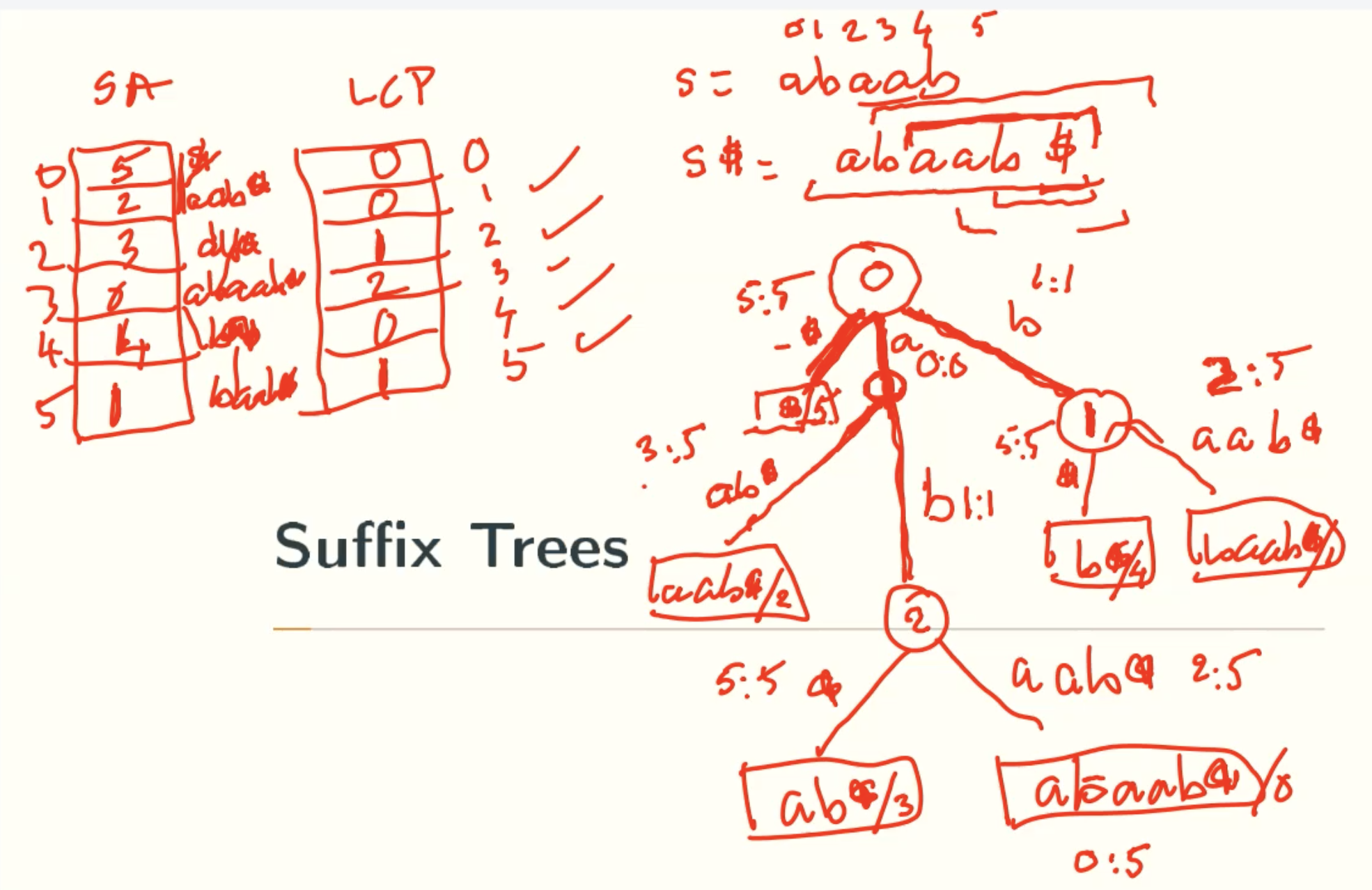
Example: abaab

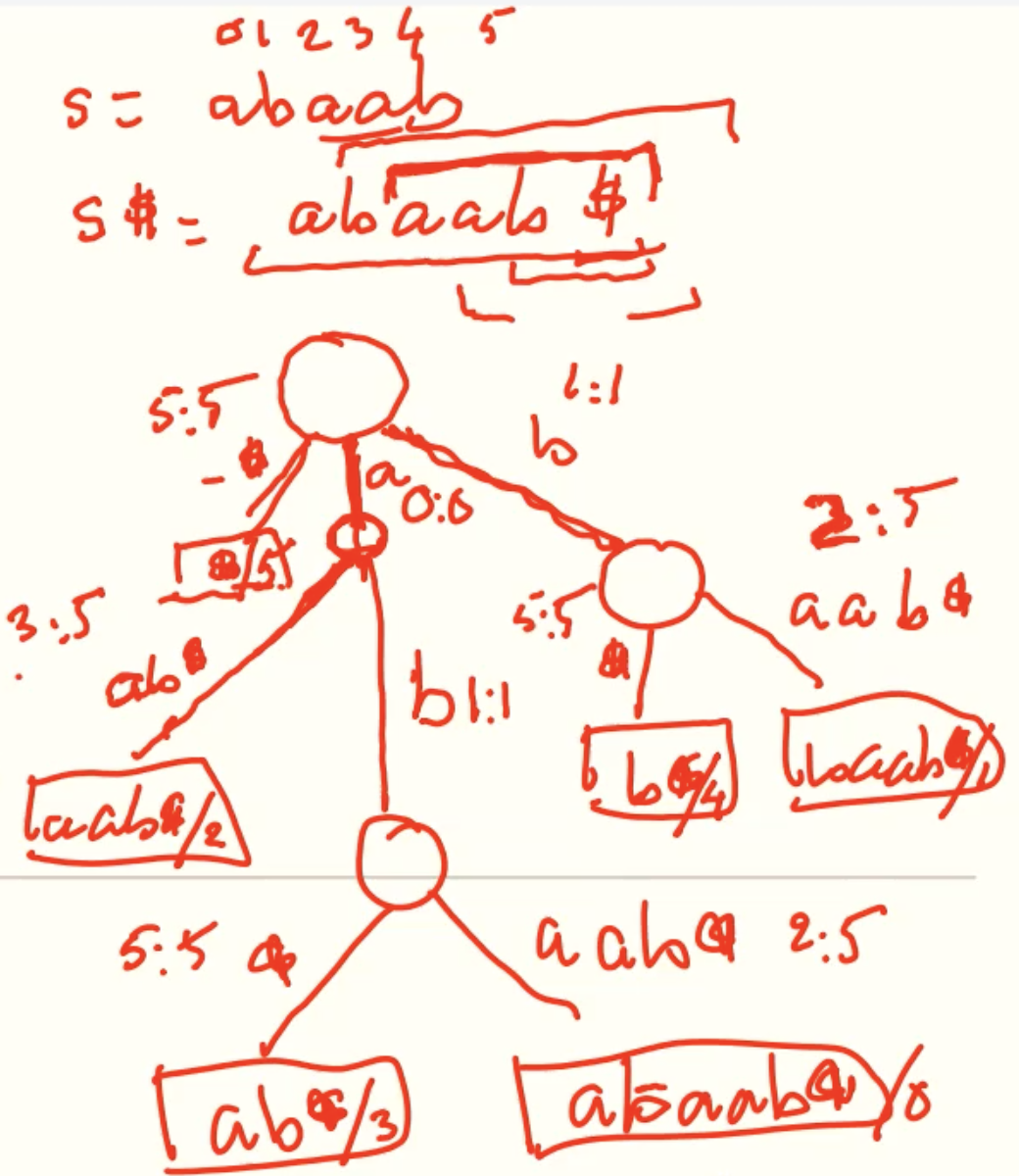
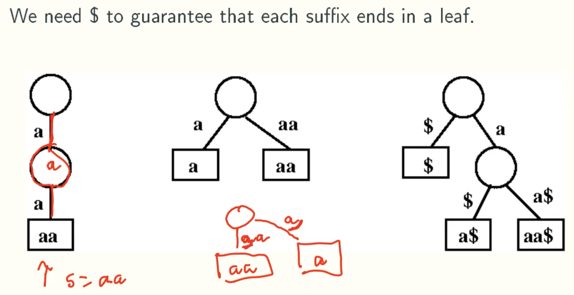
Why $?

Properties

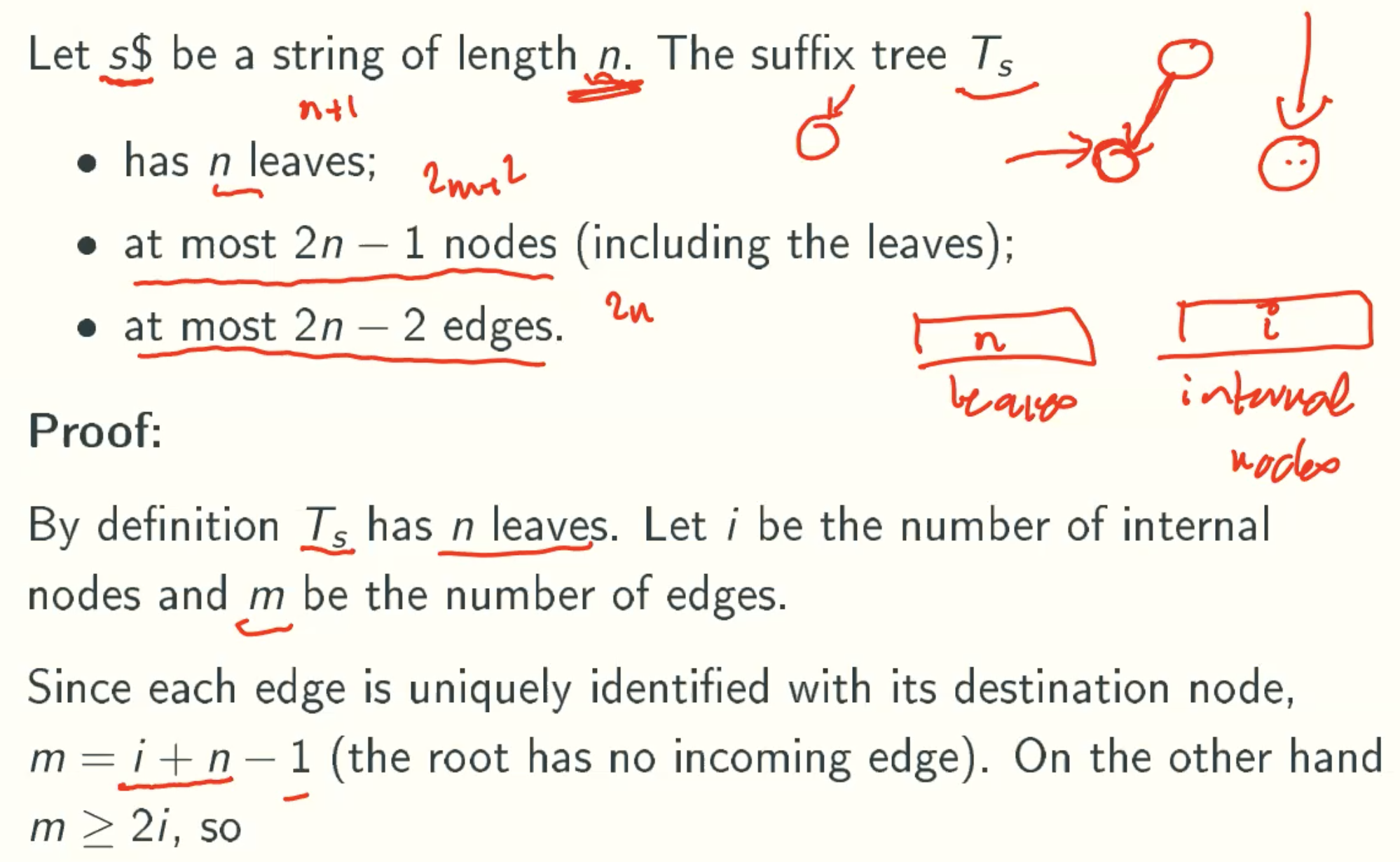
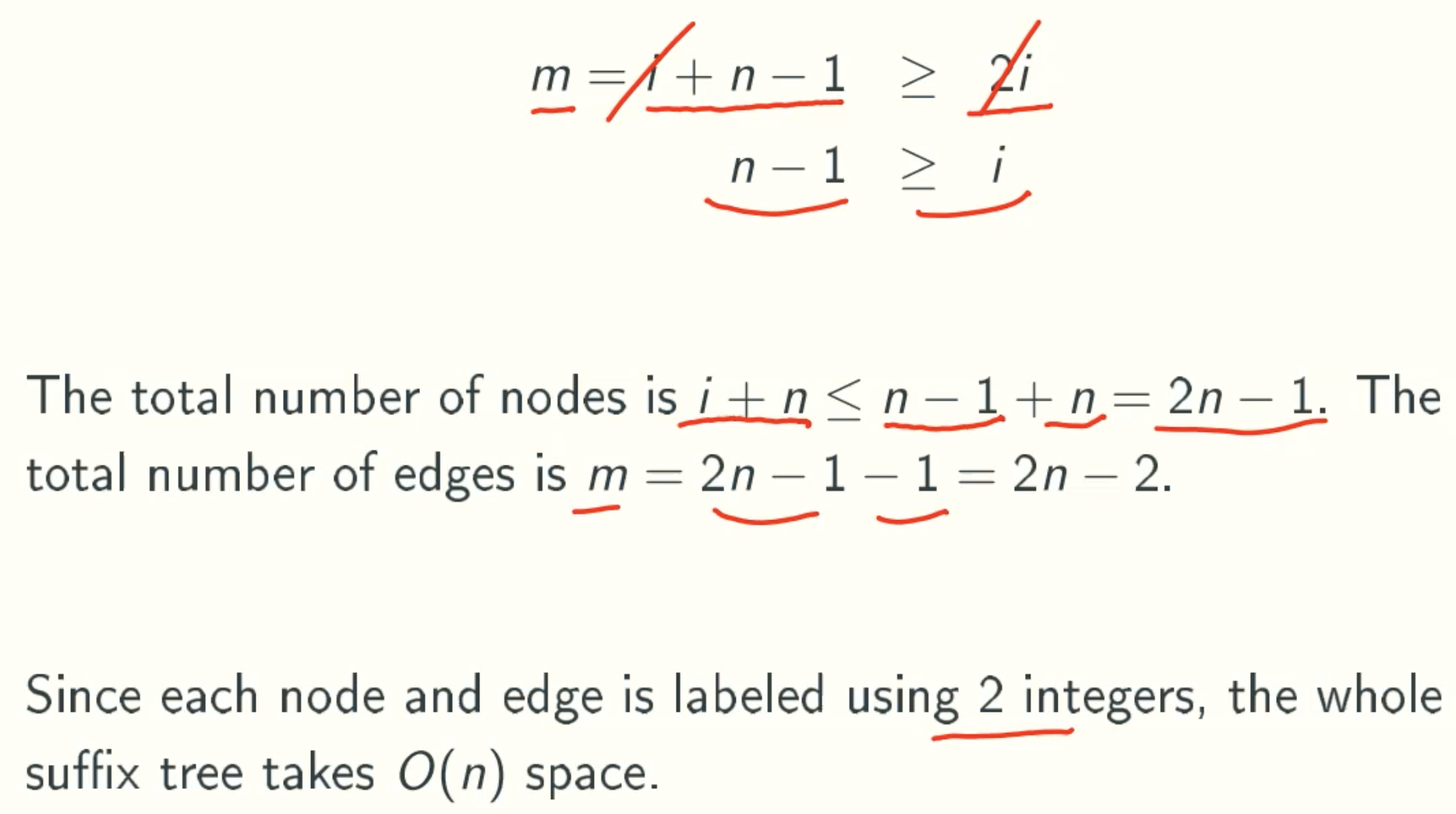
m = i + n - 1 since each node has one input except root node
m > 2i since the internal node in suffix tree must has at least 2 output

String Matching With Suffix Tree

Suffix Arrays

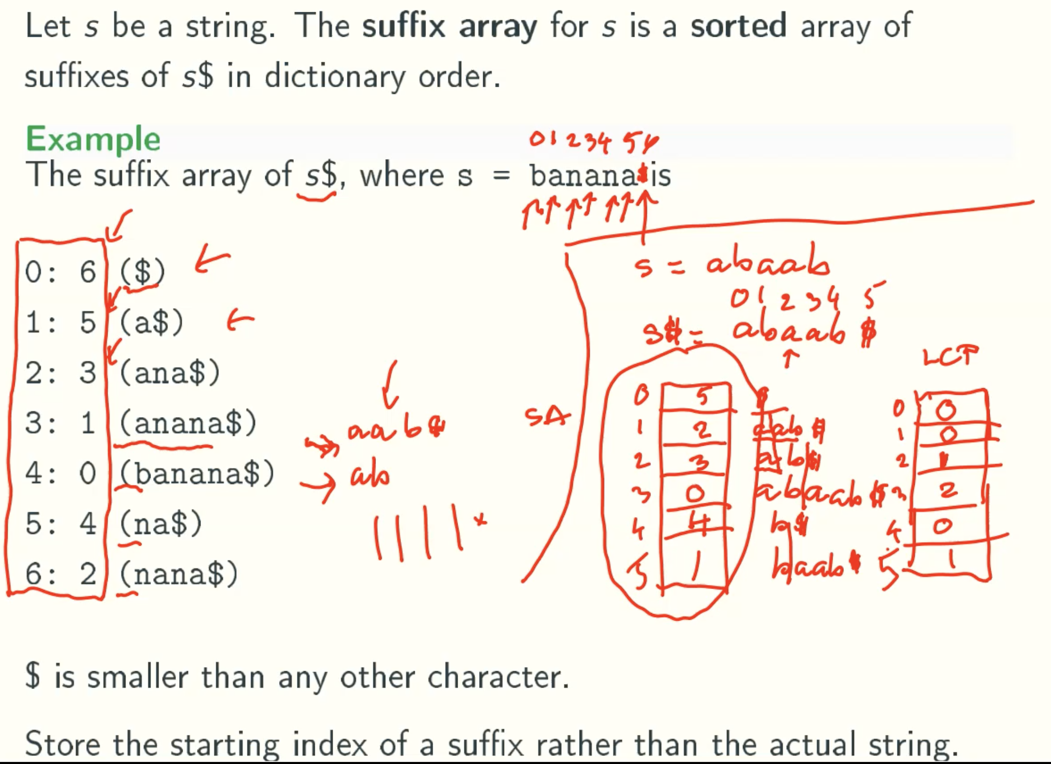
Definition

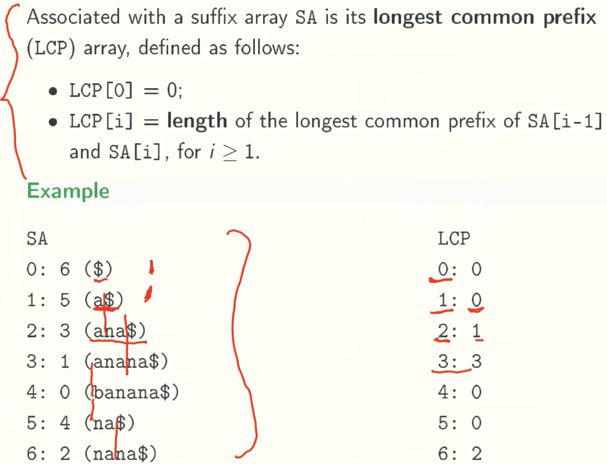
Longest Common Prefix Array

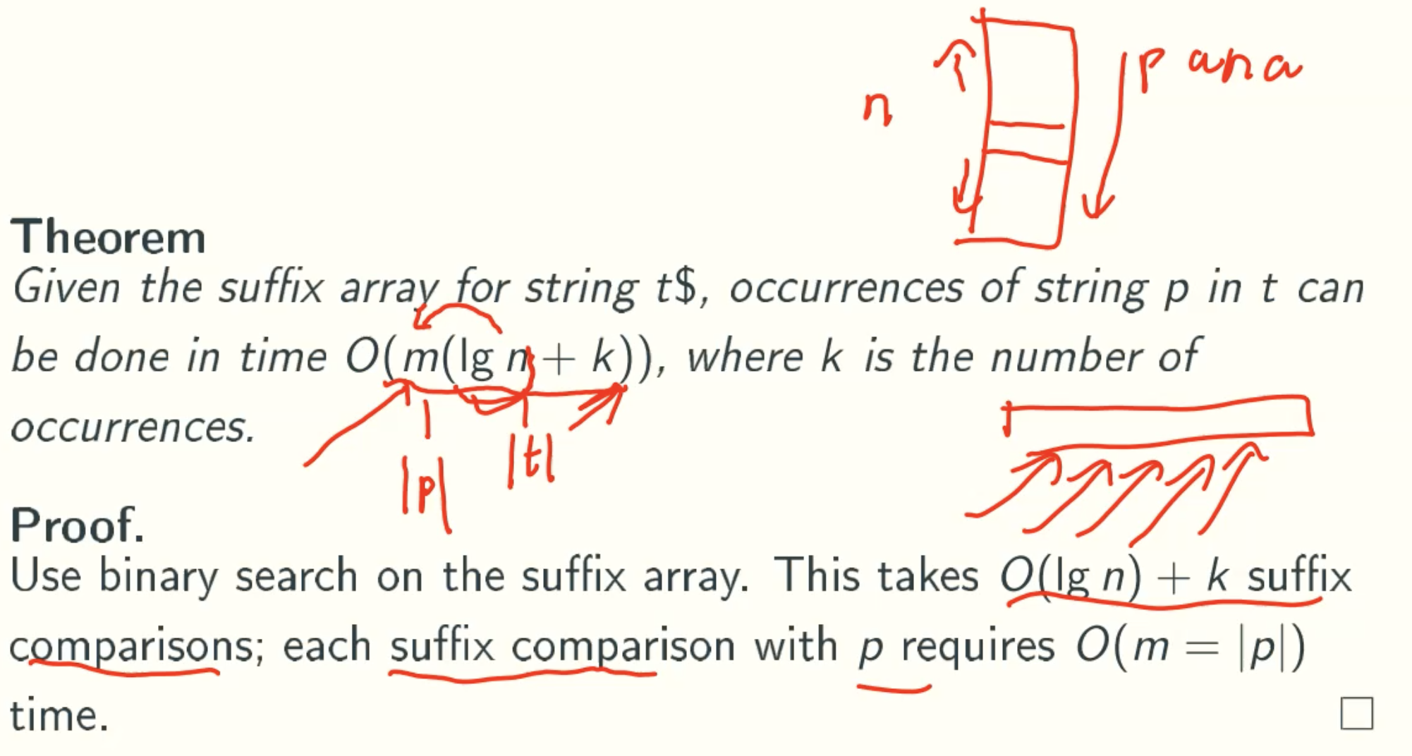
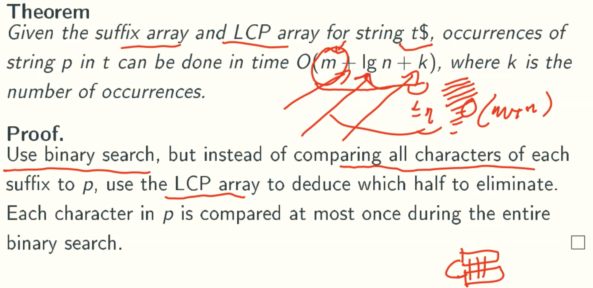
String Matching With Suffix Array

String Matching With Suffix Array And LCP Arrays

Linear-time conversions between suffix trees and suffix arrays

Suffix Tree to Suffix Arrays

Suffix Arrays to Suffix Tree

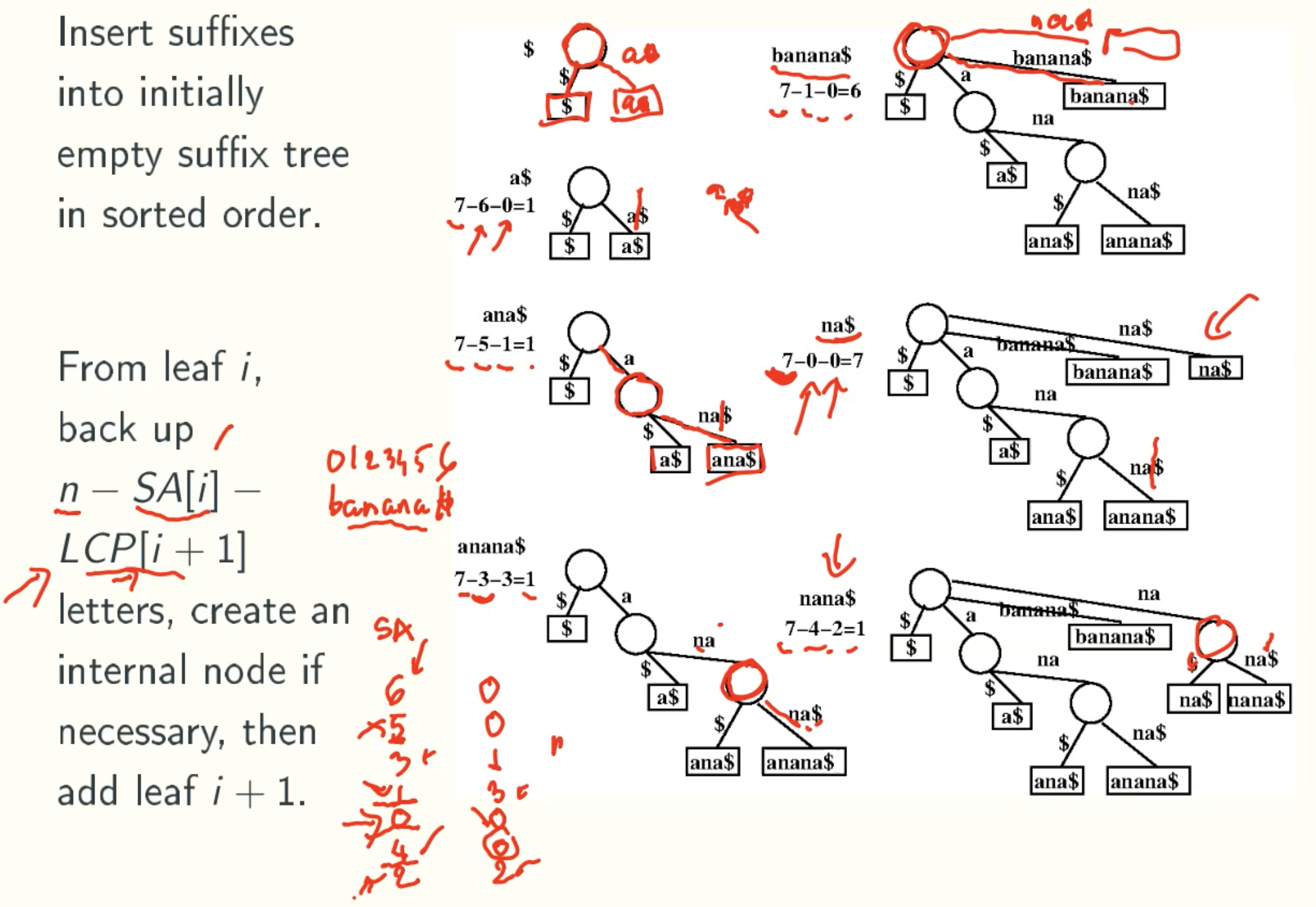
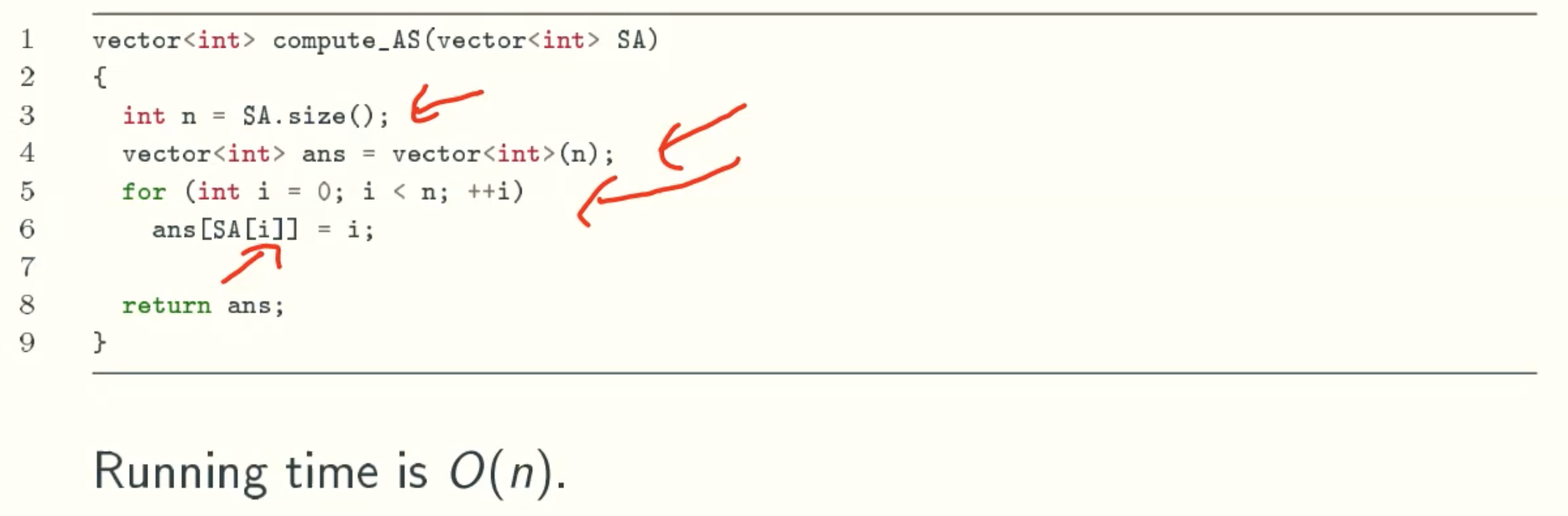
Linear-time get Suffix Arrays

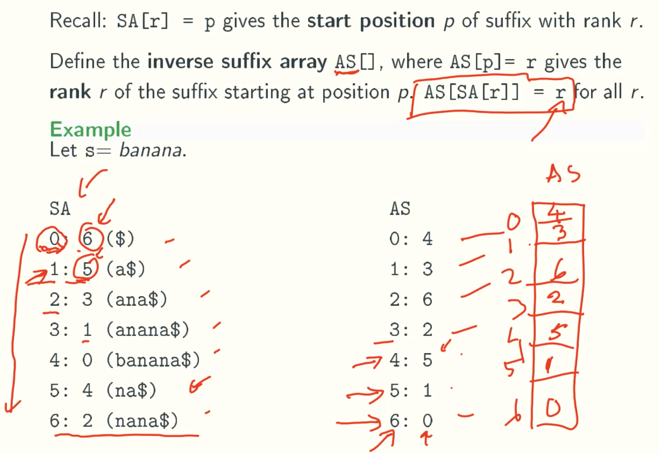
Inverse Suffix Array AS

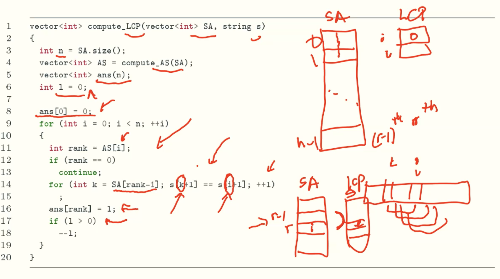
SA to LCP

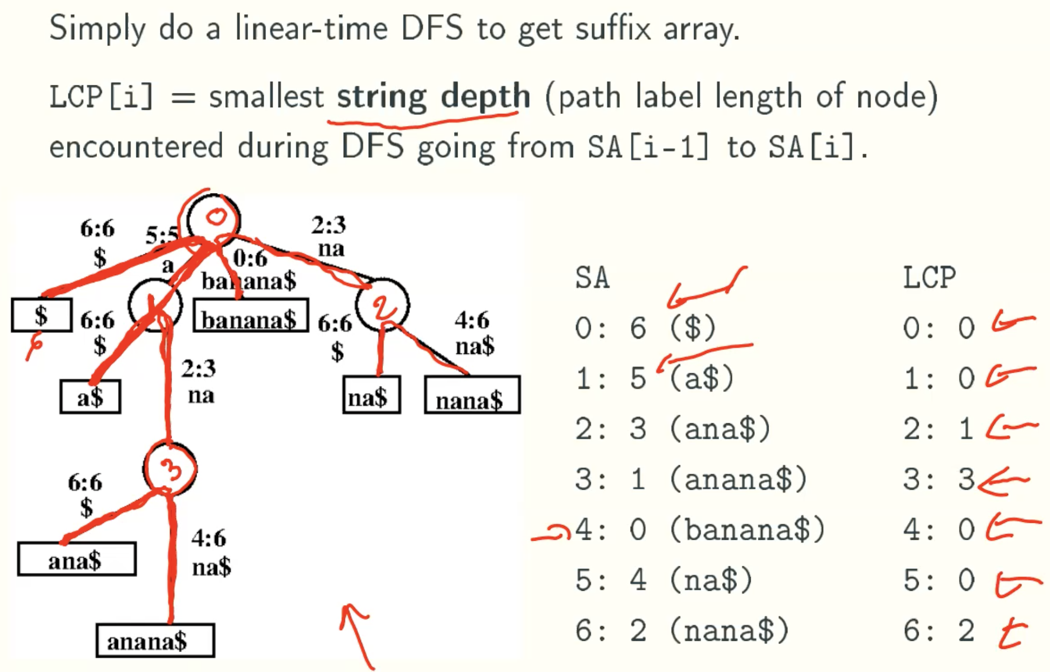
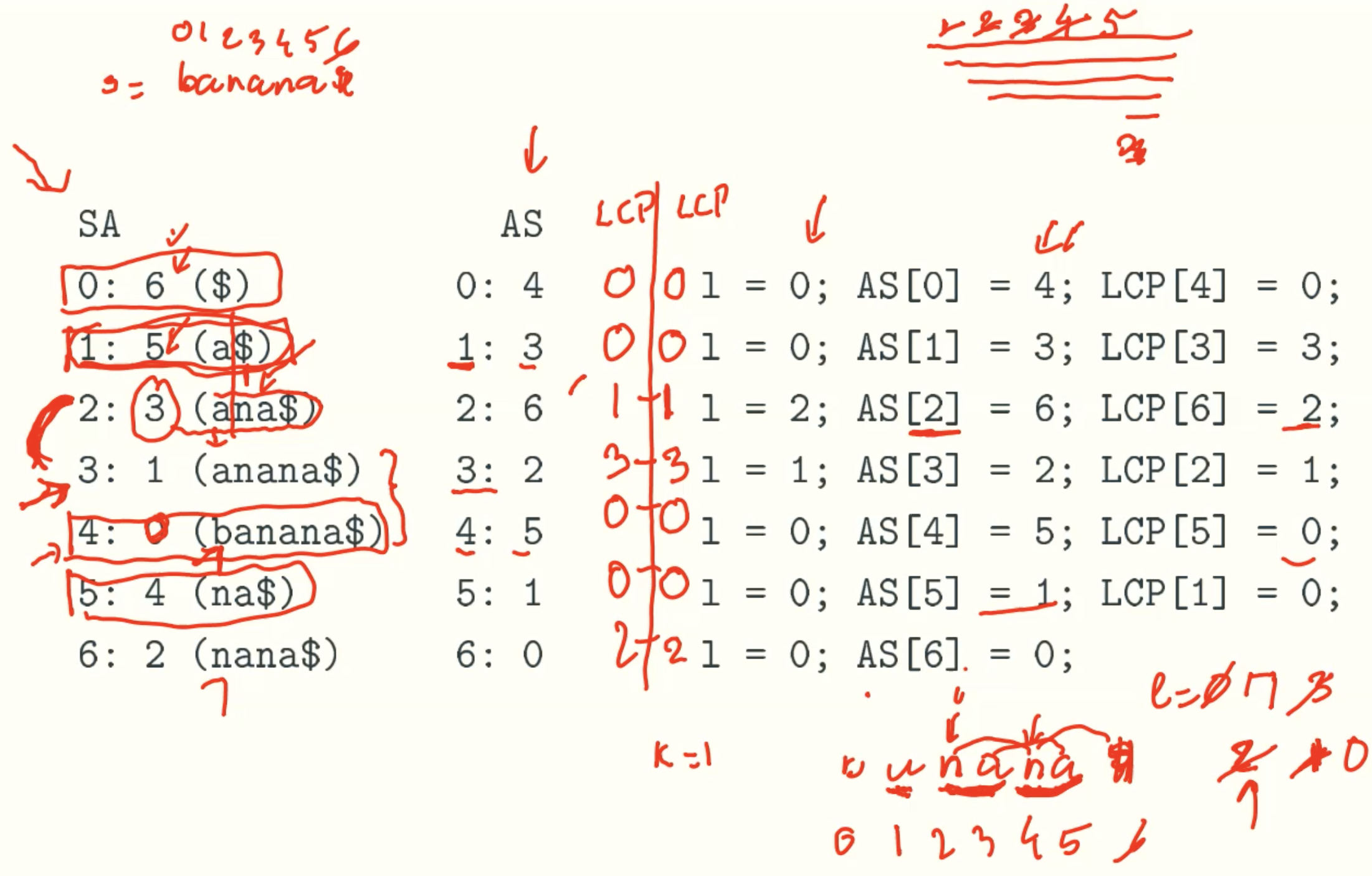
Example: banana

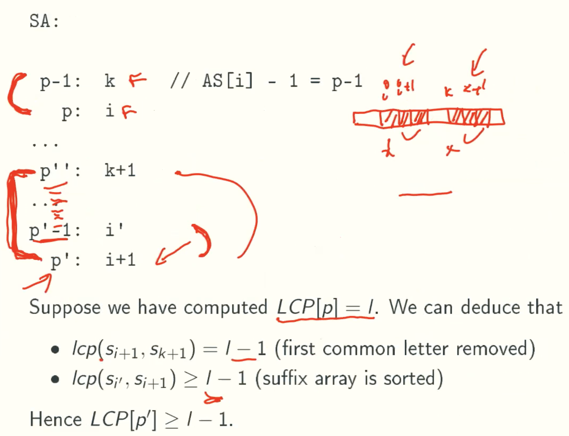
points

1. The index of AS is the start index of substring in S. Therefore, the string which start from i is the substring of the string which start from i-1.
2. If LCP[i-1] = l, which is the length of LCP of i-1. When we are comput LCP[i], there must has an string which has l-1 length common prefeix with string start from i.
   For example, banana
   when i = 1, we get LCP[1] = 3, since the length of common prefix of “anana” and “ana” is 3.
   when i = 2, the substring is “nana”, there must has an string which has 2 length common prefix with “nana” that is “na”. The reson is the lcp of “anana” and “ana” is 3. The substring of each is “nana” and “na”, they must has at least 3-1 length common prefeix. That is why we can compare from LCP[i-1]-1.
3. Because index is from 0 to n, the substring is from long to short. And from the SA rank policy, if one string is another’s prefix, the longger is in the back. So when we computing LCP from SA, the longer string will be computed first, and its LCP is guaranteed by the l value. And by the l value reducing, the lcp of shorter string which has higher rank in LCP will be smaller even 0, which is in compliance with SA rules.

Analysis

comput_LCP() makes at most 2n comparisons

• Each comparison ends in a match or a mismatch.
• Each mismatch decrements l by 1. There are n-1 mismatchs. That is because rank 0 don’t need match.
• Each match increments l by 1. Since l is bounded above by n. at most 2n matches occur.
  match - distmatch ≤ n => match ≤ dismatch + n = 2n-1
• Since l is bounded from above by n and is decreased at most n-1 times, the total running time is at most 2n.
  l increase from 0 to n and decrease from n to 0 needs 2n time

Correctness

Linear-time Construction Of Suffix Arrays

Skew Algorithm

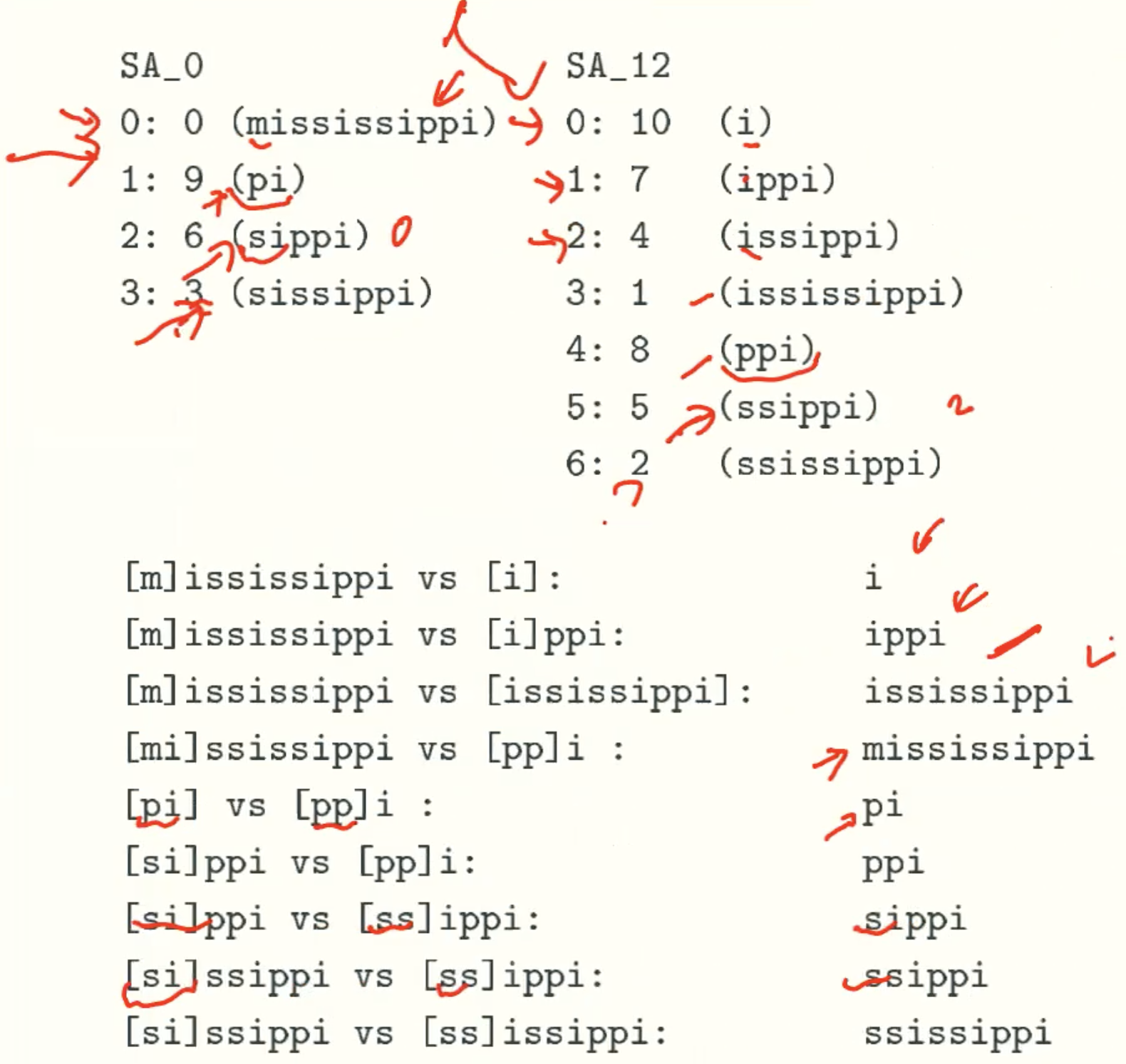
Example: mississippi

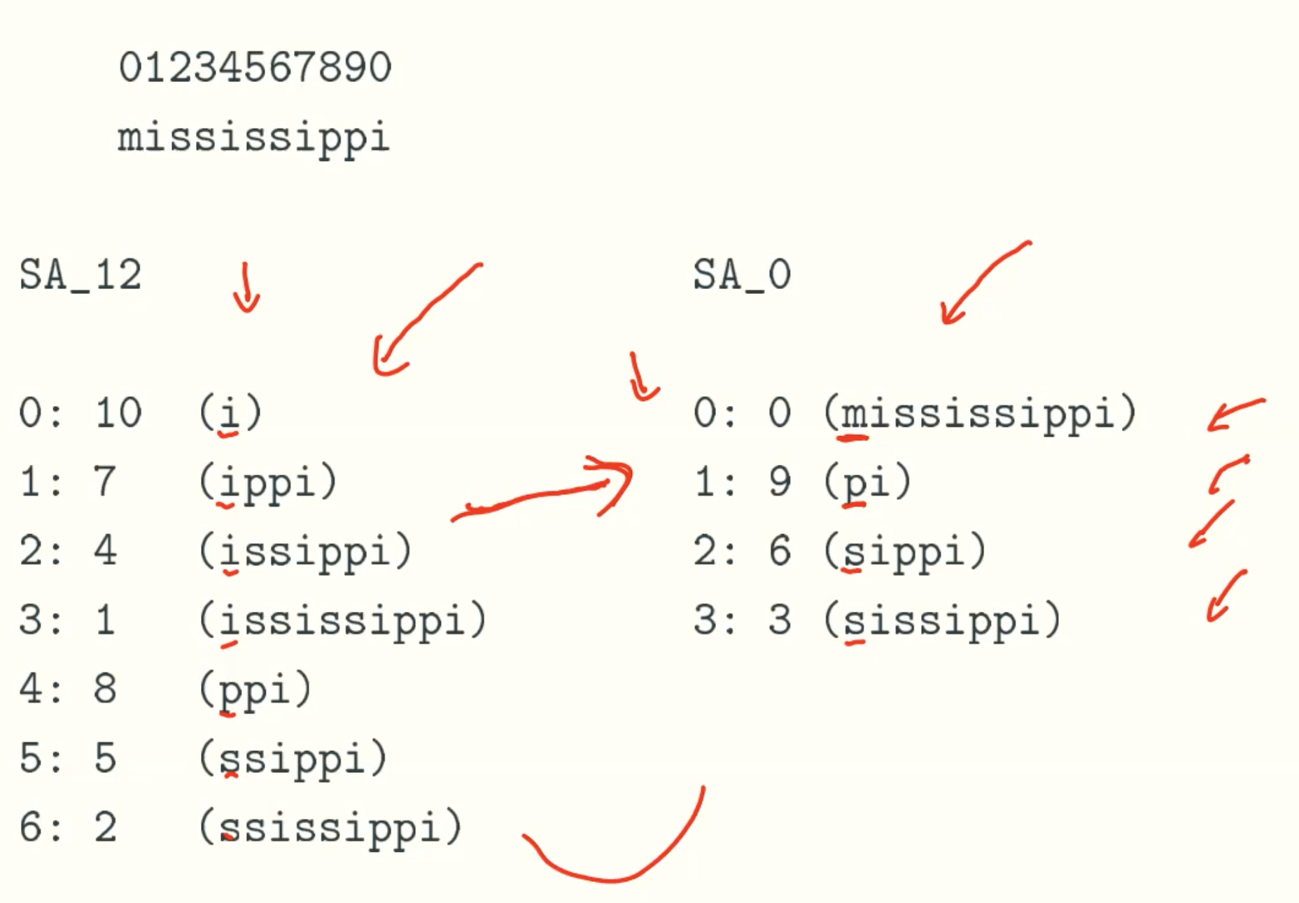
SA₁₂ to SA₀

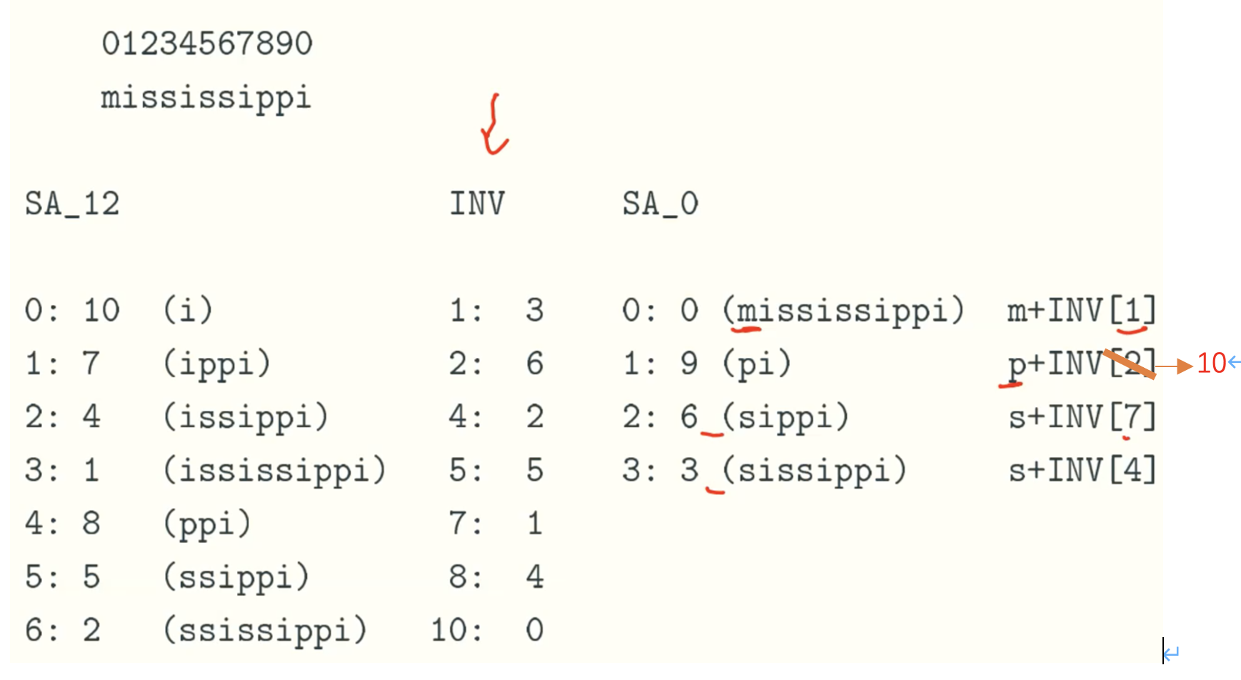
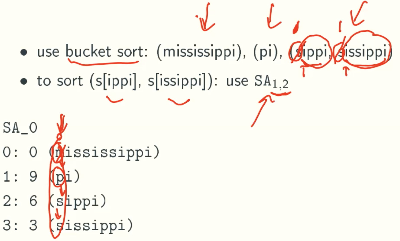
m+INV[1] = “m3”, p+INV[10] = “p0”, s+INV[7] = “s1”, s+INV[4] = “s2”, then we sort this four string get the rank of SA0 which need linear time, because each string just has two digit.

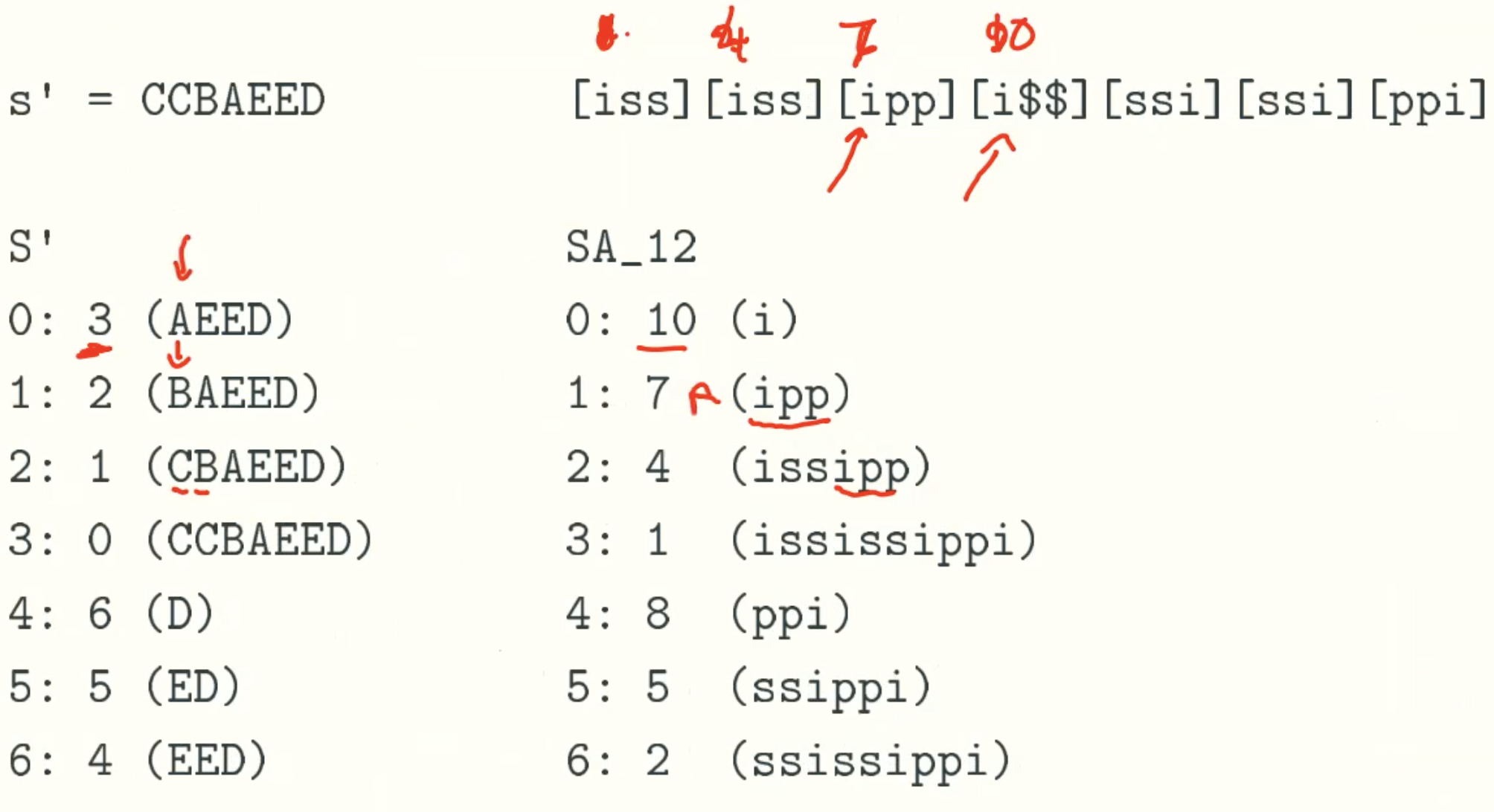
Construct SA₁₂ recursively

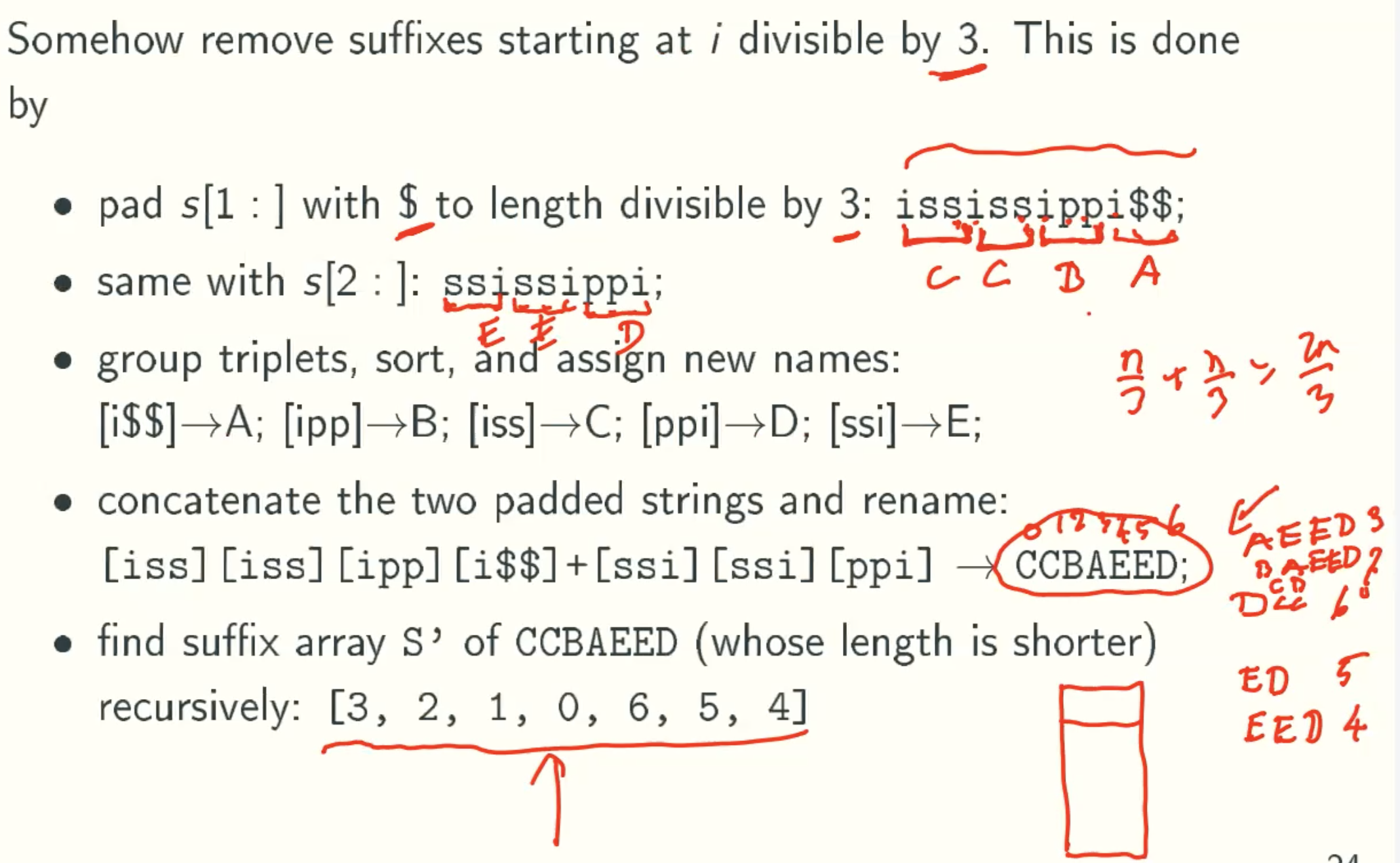
Change back

Constuct SA₀

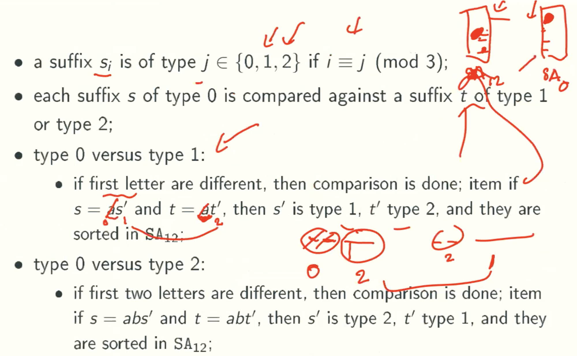
Merging SA₀ and SA₁₂ In Linear Time

Example